make.lake
make.lake will modify an initial topobathymetric surface to add new water areas based on user-provided contours. This may be of use in areas that have bathymetric surveys in the form of contours. The following is typical usage for make.lake.
Prepare a topography file as a geotif.
Prepare or obtain a polyline shapefile that contains depth contours of the lake. Ensure that the geotif and shapefile have the same coordinate system.
Run
make.laketo generate input files for D-Claw. Inspect the output and adjust any input parameters as needed.Using these files, set up a D-Claw simulation to run and analyze.
diggerwill not do this for you.
A code snippet that uses make.lake may be found in the file digger/examples/pre-run/black_lake/make_lake_black_lake_example.py. In this example, a DEM from the U.S. Geological Survey (2017) is adjusted to include depth data based on contours from Black Lake, Washington (Washington State Department of Ecology, 2022).
"""An example of using digger.make.lake.

This example uses Black Lake topography and provides an example of using
digger.make.lake.
"""

import yaml

from digger import make

# Run digger.make.lake

black_lake_info = make.lake(
    topo_path="../../../data/black_lake_dem.tif",
    lake_contour_path="../../../data/black_lake_contours.shp",
    depth_field="Depth",
    b_prefix="b_black_lake",
    eta_prefix="eta_black_lake",
    fig_path="black_lake.png",
)

# Save lake info to a yaml file
with open("black_lake_info.yaml", "w") as file:
    yaml.dump(black_lake_info, file, sort_keys=False)
After this code runs, it will produce geotif and topotype3 files that specify the modified topobathymetry.
It will also create diagnostic figures.
The standard diagnostic figure from make.lake
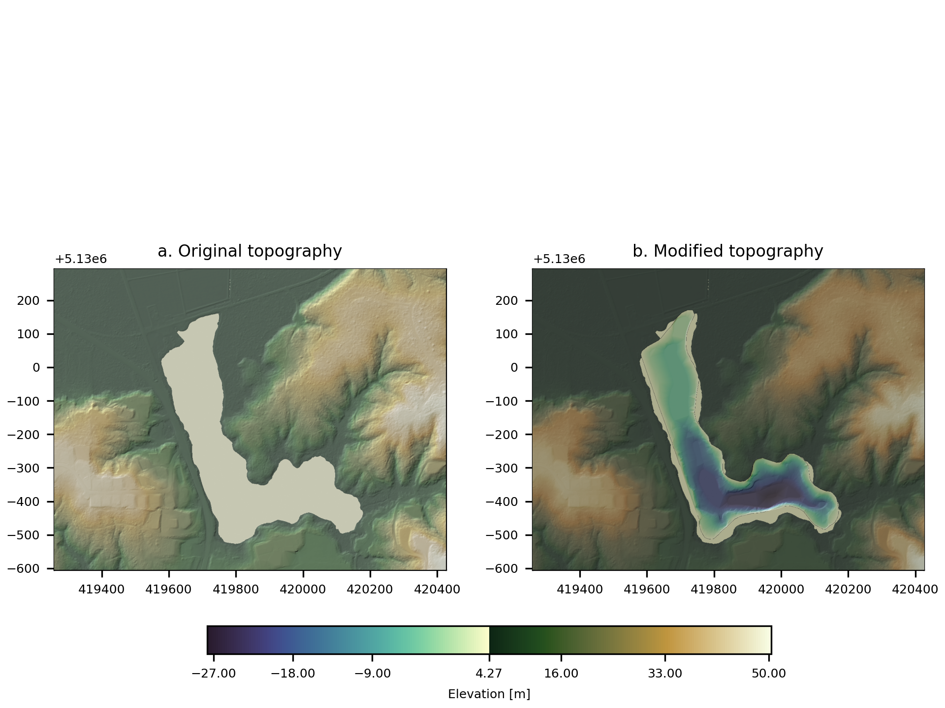
Fig. 5 An example of the diagnostic output provided by digger.make.lake.
A dictionary containing some diagnostic information is returned. It contains the following elements:
x1: 419582.1993265635
x2: 420170.46798666567
y1: 5129487.699441308
y2: 5130169.700250362
lake_surface_height: 4.2670063972473145
Another example may be found in the file digger/examples/pre-run/synthetic/make_lake_synthetic_example.py. In this example, a synthetic lake is placed into flat topography.
"""An example of using digger.make.lake.

This example uses synthetic topography and provides an example of using
digger.make.lake.
"""

import geopandas as gpd
import matplotlib.pylab as plt
import numpy as np
import pandas as pd
import rasterio
import shapely
import yaml

from digger import make


# Define the herbie function (Lee and others, 2011) as a means
# to generate contours.
# Lee, H., Gramacy, R., Linkletter, C., and Gray, G., 2011, Optimization
# subject to hidden constraints via statistical emulation. Pacific Journal
# of Optimization, 7(3), 467-478, last accessed June 5, 2025 at
# http://www.ybook.co.jp/online2/oppjo/vol7/p467.html
def herbie(X, Y):
    # standard herbie:
    Z = (
        np.exp(-((X - 1) ** 2))
        + np.exp(-0.8 * (X + 1) ** 2)
        - 0.05 * np.sin(8 * (X + 0.1))
    )
    Z += (
        np.exp(-((Y - 1) ** 2))
        + np.exp(-0.8 * (Y + 1) ** 2)
        - 0.05 * np.sin(8 * (Y + 0.1))
    )
    # additional adjustments to turn herbie into a lake with
    # edges
    Z *= 10
    Z -= 15
    Z[Z < 0] = 0
    return Z


# For illustration purposes, we need to make a raster representing the lake
# we will then write it out as a shapefile and the shapefile to generate
# a lake. In more typical application, the shapefile would be derived from
# surveys.
x = np.linspace(-5, 5, 201)
y = np.linspace(-5, 5, 201)
X, Y = np.meshgrid(x, y)
Z = herbie(X, Y)
clines = np.arange(0, 7, 1)  # contour lines to plot and save

fig, ax = plt.subplots(1, 1, dpi=300)
cs = ax.contour(X, Y, Z, clines, cmap="viridis", linewidths=0.5)
ax.axis("equal")
ax.set_title("Lake Herbie")
cbar = fig.colorbar(cs)
fig.savefig("herbie_contours.png")

# Create a topography file
transform = rasterio.transform.from_bounds(X.min(), Y.min(), X.max(), Y.max(), *Z.shape)
with rasterio.open(
    "lake_herbie_topography.tif",
    "w",
    driver="GTiff",
    height=Z.shape[0],
    width=Z.shape[1],
    count=1,
    dtype=Z.dtype,
    # crs='+proj=latlong',
    transform=transform,
) as sink:

    # Set the topography for lake herbie to zero everywere.
    sink.write(Z * 0, 1)


# Write Lake Herbie to a shapefile
records = []
geometries = []

# Loop through contour levels and extract contours using
# rasterio.features.shapes.
# This is a slightly different method than using the matplotlib contours
# but is a more reliable method for generating shapefiles from raster contours.
for level in clines:
    mask = Z > level
    features = rasterio.features.shapes(mask.astype(rasterio.int8), transform=transform)

    for polygon_mapping, _ in features:
        polygon = shapely.geometry.shape(polygon_mapping)
        lines = []
        lines.append(polygon.exterior)
        lines.extend(polygon.interiors)
    for line in lines:

        geometries.append(shapely.LineString(line))
        records.append({"level": float(level)})

gdf = gpd.GeoDataFrame(
    pd.DataFrame(records),
    geometry=geometries,
)
gdf.to_file("lake_herbie.shp")

# Run digger.make.lake
lake_info = make.lake(
    topo_path="lake_herbie_topography.tif",
    lake_contour_path="lake_herbie.shp",
    depth_field="level",
    depth_unit_convert=1.0,
    write_tif=True,
    write_tt3=False,
    fig_path="lake_herbie.png",
)

# Save lake info to a yaml file
with open("lake_info.yaml", "w") as file:
    yaml.dump(lake_info, file, sort_keys=False)
In this example, we generated a lake from the following synthetic contour set:
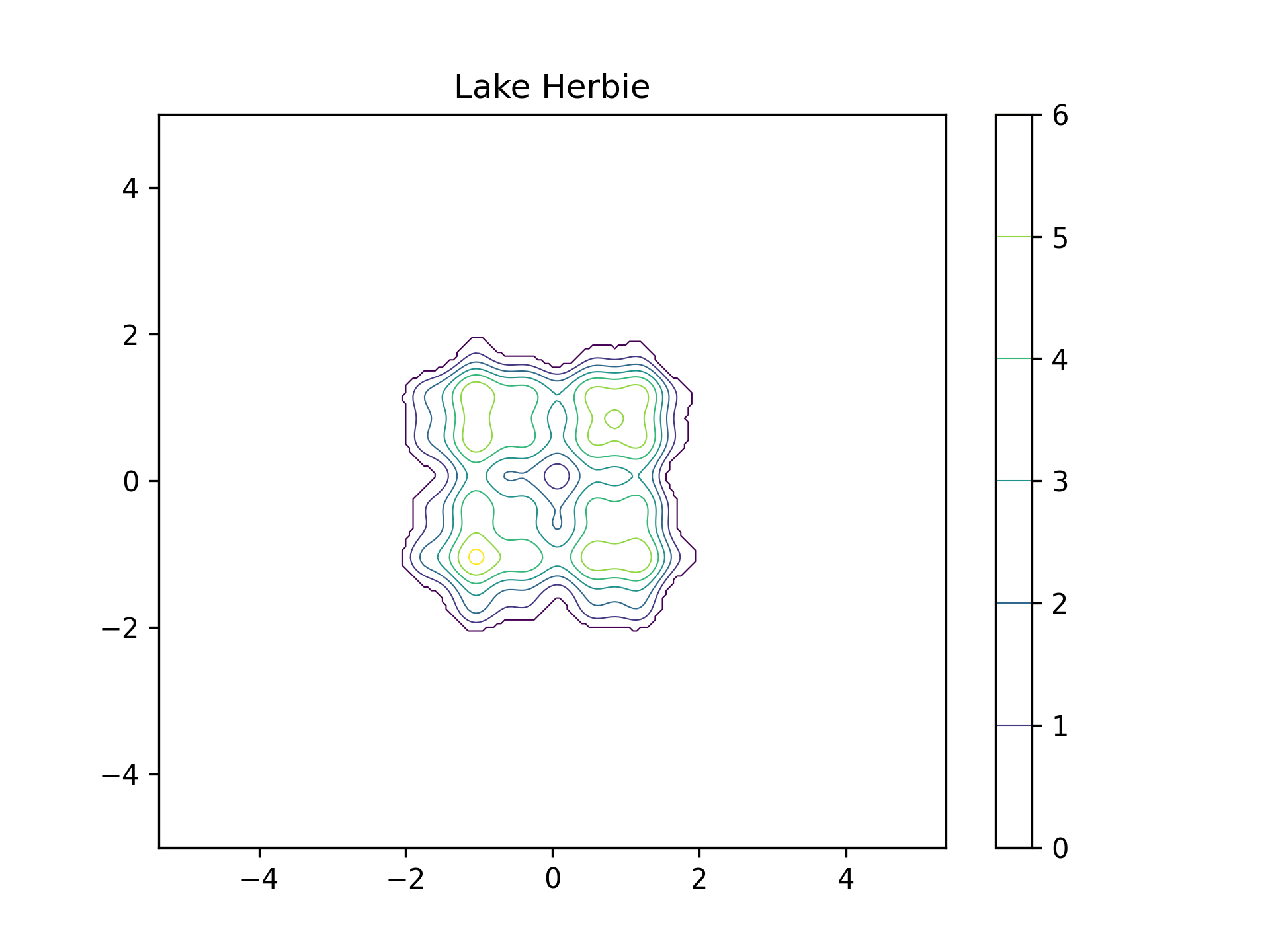
Fig. 6 The contour set used by make.lake
The standard diagnostic figure from make.lake
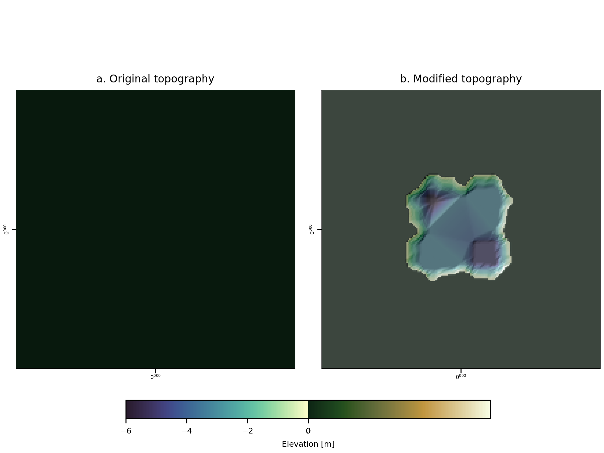
Fig. 7 An example of the diagnostic output provided by digger.make.lake.
A dictionary containing some diagnostic information is returned. It contains the following elements:
x1: -2.014925373134328
x2: 1.9154228855721396
y1: -1.9154228855721396
y2: 2.014925373134328
lake_surface_height: 0.0
References
Black Lake Bathymetry: Washington State Department of Ecology, 2022, Lake Bathymetry Contour Lines, Accessed on September 4, 2025, at https://geo.wa.gov/datasets/waecy::lake-bathymetry-contour-lines/explore?location=46.316320%2C-124.040184%2C16.84.
Black Lake DEM U.S. Geological Survey, 2017, USGS one meter WA Olympic Peninsula C2 2017, Accessed on September 4, 2025, at https://prd-tnm.s3.amazonaws.com/index.html?prefix=StagedProducts/Elevation/1m/Projects/WA_Olympic_Peninsula_C2_2017/TIFF/.