compare.confusion

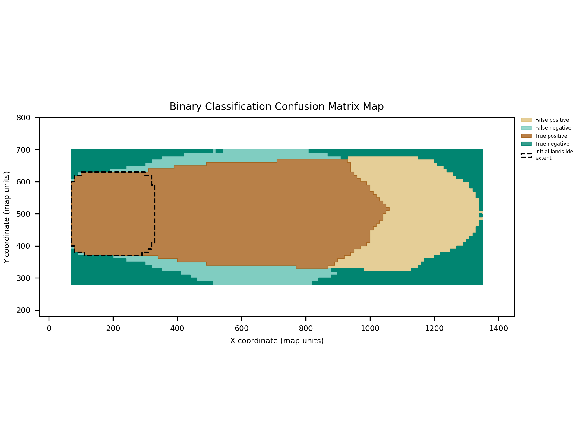
The function compare.confusion compares the observed extent of landslide impact with a simulated extent. It classifies each location within the region of interest into the four elements of the binary classification confusion matrix:

Table 1 Elements of the binary classification confusion matrix

Name	Description
True Positive	Observed and predicted as true
False Positive	Observed as false but predicted as true
True Negative	Observed and predicted as false
False Negative	Observed as true but predicted as false

An example of using this functionality is provided in the file digger/examples/post-run/synthetic/setpostprocess.py.

# Postprocess the synthetic example
from digger import compare
from digger.utils.fgtools import fg2shp

# Convert the extent of observed landslide impact into a shapefile
fg2shp(
    filein="_output/fgmax0001.txt",
    fileout="fgmax-h_max.shp.zip",
    varname="h_max",
    fgtype="fgmax",
    contours=[0],
    geom_type="MultiPolygon",
)

# Convert the initial timestep into a shapefile, this is
# used to depict the initial landslide extent on the plot.
fg2shp(
    filein="_output/fgout0001.b0001",
    fileout="t0-h.shp.zip",
    varname="h",
    fgtype="fgout",
    contours=[0],
    geom_type="MultiPolygon",
)

# To conduct a binary classification analysis, we need a 'True' extent of
# landslide runout. Such an extent is typically based on observations.
# Because this is a synthetic example, here we will make an example polygon
# that is based on another simulation that used different parameters
# (depth=5 and kappita=1e-8 rather than depth=2 and kappita=1e-10).
# The resulting extent from this other simulation is located within the file
# ../../../data/fgmax-h_max-truth.shp.zip

# Optionally we could make a shapefile indicating the region to consider for
# confusion analysis. The entire extent of the region influence the total
# number of true negatives. If this is not provided, the bounding envelop of the
# simulation and true shapes is used.

# Conduct confusion analysis
# Note that we can mix and match shapefiles and geojson. We must use OGR standard
# filetypes that fiona can read.
confusion_info = compare.confusion.extract_shapes(
    truth_fn="../../../data/fgmax-h_max-truth.shp.zip",
    simulation_fn="fgmax-h_max.shp.zip",
    initial_source="t0-h.shp.zip",
)

metrics = compare.confusion.calculate_metrics(**confusion_info)

Attention

This code snippet is not fully self-sufficient. This snippet relies on simulation output files. To reproduce the example, execute the file digger/examples/post-run/synthetic/setpostprocess.py from within the directory in which it is located. Before the script is executed either the example simulation must be run or the file digger/data/synthetic_output.zip must be unzipped and the resulting directory (_output) must be placed within digger/examples/post-run/synthetic/.

This code generates a diagnostic figure that visualizes the confusion matrix.

Fig. 16 An example of the diagnostic output provided by digger.calculate.confusion.

It also generates a yaml file containing all of the calculated metrics. See the function API for an explanation of each metric.

ppv: 0.7226582940868654
tpr: 0.8395136778115502
tnr: 0.49185043144774687
npv: 0.6602316602316602
fnr: 0.16048632218844985
fpr: 0.5081495685522531
fdr: 0.27734170591313445
for: 0.33976833976833976
f1: 0.7767154105736782
ts: 0.6349425287356322
accuracy: 0.7046130952380952
alphaT: 0.6349425287356322
betaT: 0.12137931034482759
gammaT: 0.24367816091954023
OmegaT: 0.26988505747126434
modifiedOmegaT: 0.3650574712643678