Command Line Plotting

The USGS Slab Models repository provides several options for visualizing slab geometry models. Users may choose to make maps of slab depth, dip, strike, thickess, and uncertainty. There are also options for plotting slab cross-sections and even comparing slab models to one another.

Create a Slab Model Map

To make a 2-dimensional map of a slab model, navigate to src/plotting/ and activate the Python environment. Next, use the following command:

python make_plots.py -f [file] [-t type] [-o outfile] [-c compare_file] [-p clipping_mask] [-x xsec] [-i input_file] [-n name] [--contours]

Required Arguments

• -f --file

  path to the file to be plotted. e.g. ../output/exp_slab2_04-18/exp_slab2_dep_04-18.grd

Optional Arguments

• -t --type

  Specifies type of plot to make. 2D or 3D.

• -o --outfile

  Specifies file name to save figure to.

• -c --compare

  Optional second model to compare with. e.g. ../output/exp_slab2_08-24/exp_slab2_dep_08-24.grd

• -p --clip

  Path to clipping file for selected model. Required for cross-sections. e.g. ../output/exp_slab2_04-18/exp_slab2_clp_04-18.csv

• -x --xsec

  Option for plotting cross-sections. Must specify the ‘lon,lat,az’ for the cross-section line.

• -i --input

  Path to input data to add to plot. e.g. ../../input/input_files/04-18/exp_04-18_input.csv

• -n --name

  Figure title.

Examples

The following section illustrates the use of the above options by giving some examples for the available features.

Basic 2D Plot

Only specifying the required --file flag will generate a simple 2D visualization.

python make_plots.py -f ../output/cas_slab2_04-18/cas_slab2_surf_dep_04-18.grd

Cascadia slab surface model plot.

Use the --contours flag to add contours to the figure.

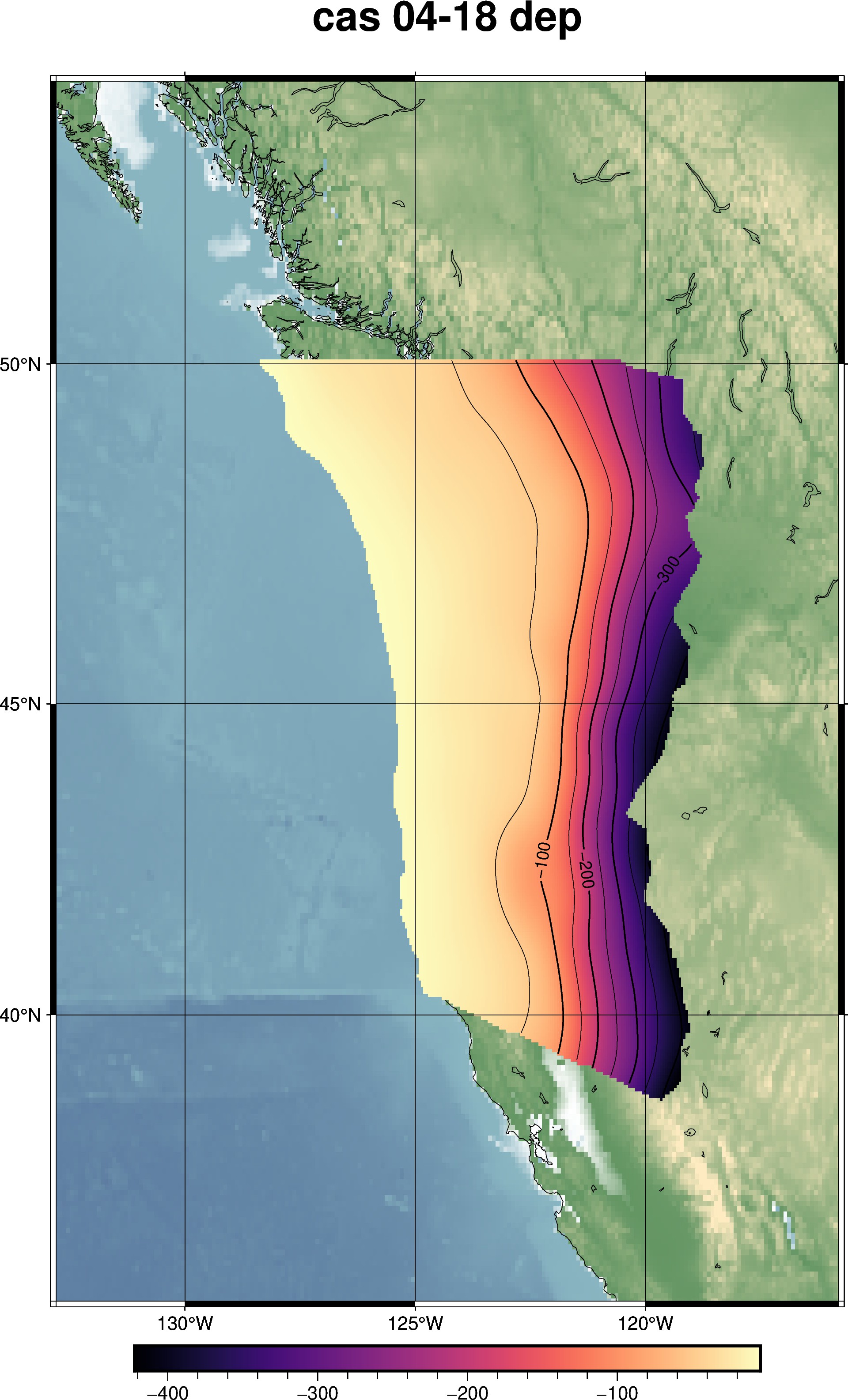
Cascadia slab surface model plot with contour lines.

3D Plot

To make a 3D plot, the option can be specified using the --type flag.

python make_plots.py -f ../output/cas_slab2_04-18/cas_slab2_surf_dep_04-18.grd -t 3D

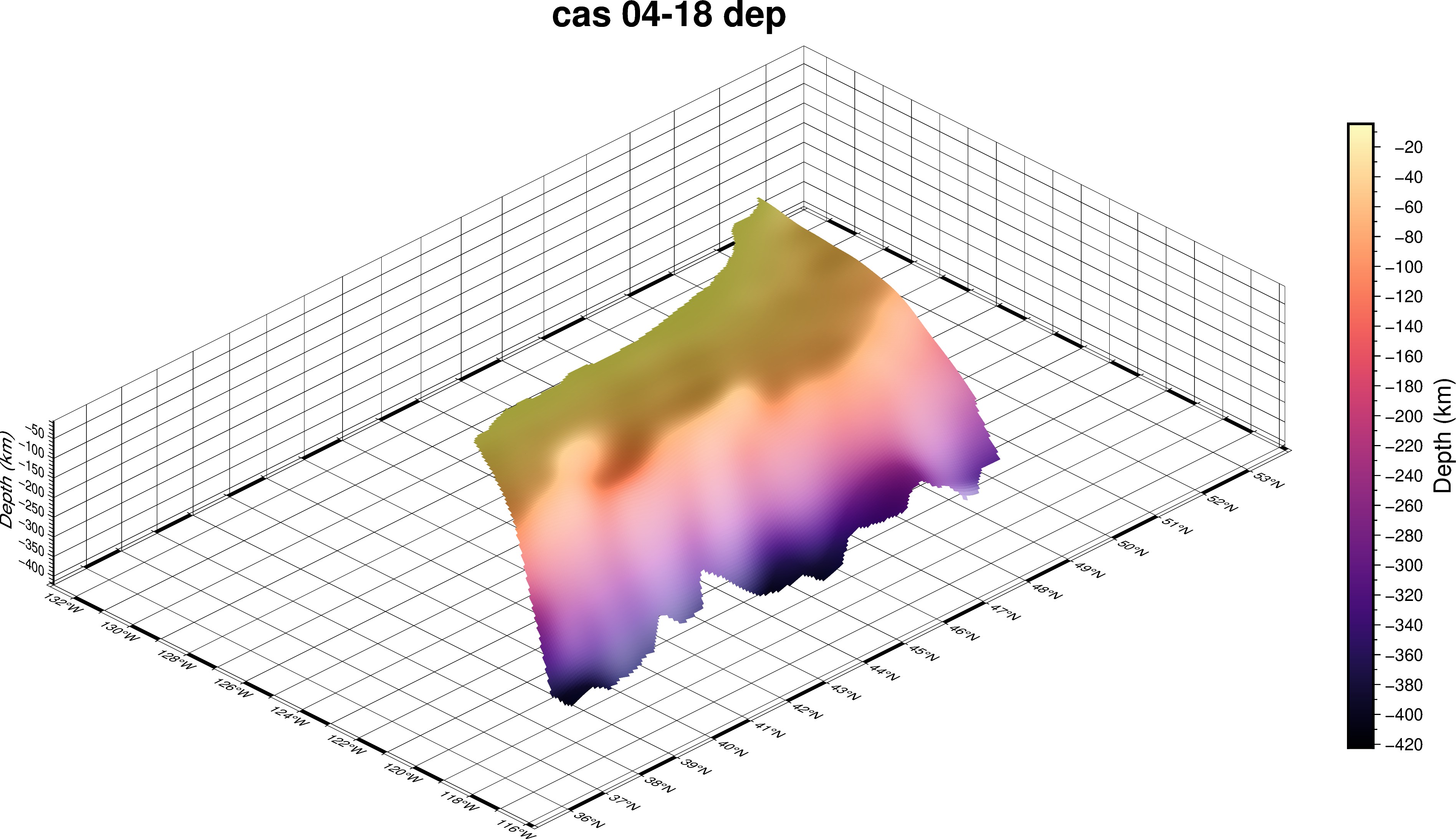
Cascadia slab surface model 3D plot.

Cross-Section Plotting

Cross-section plots can be made by using the --xsec flag and specifying the longitude, latitude, and azimuth angle of the section. Note the clipping mask must also be specified to constrain the line extent using the --clip flag.

python make_plots.py -f ../output/cas_slab2_04-18/cas_slab2_surf_dep_04-18.grd -x 227,45,90 -p ../output/cas_slab2_04-18/cas_slab2_surf_clp_04-18.csv

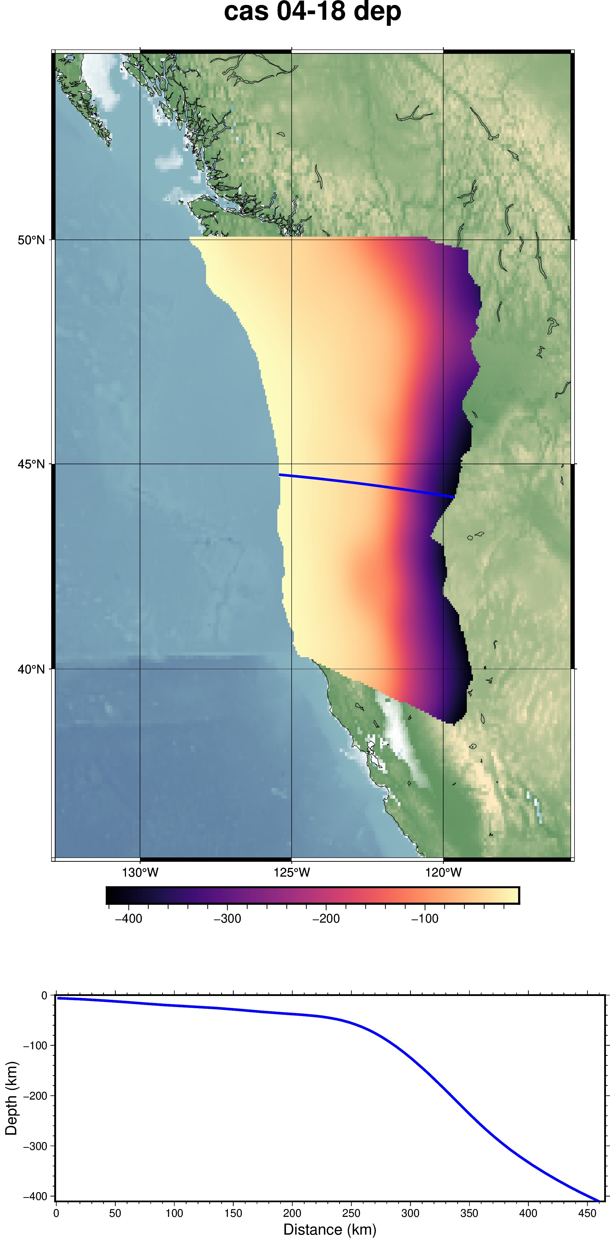
Cascadia surface cross-section.

Adding Input Data

Overlaying the input data used to constrain a slab model can be accomplished by using the --input flag, followed by the path to the appropriate input file.

python make_plots.py -f ../output/cas_slab2_04-18/cas_slab2_surf_dep_04-18.grd -i ../../input/input_files/04-18/cas_04-18_input.csv

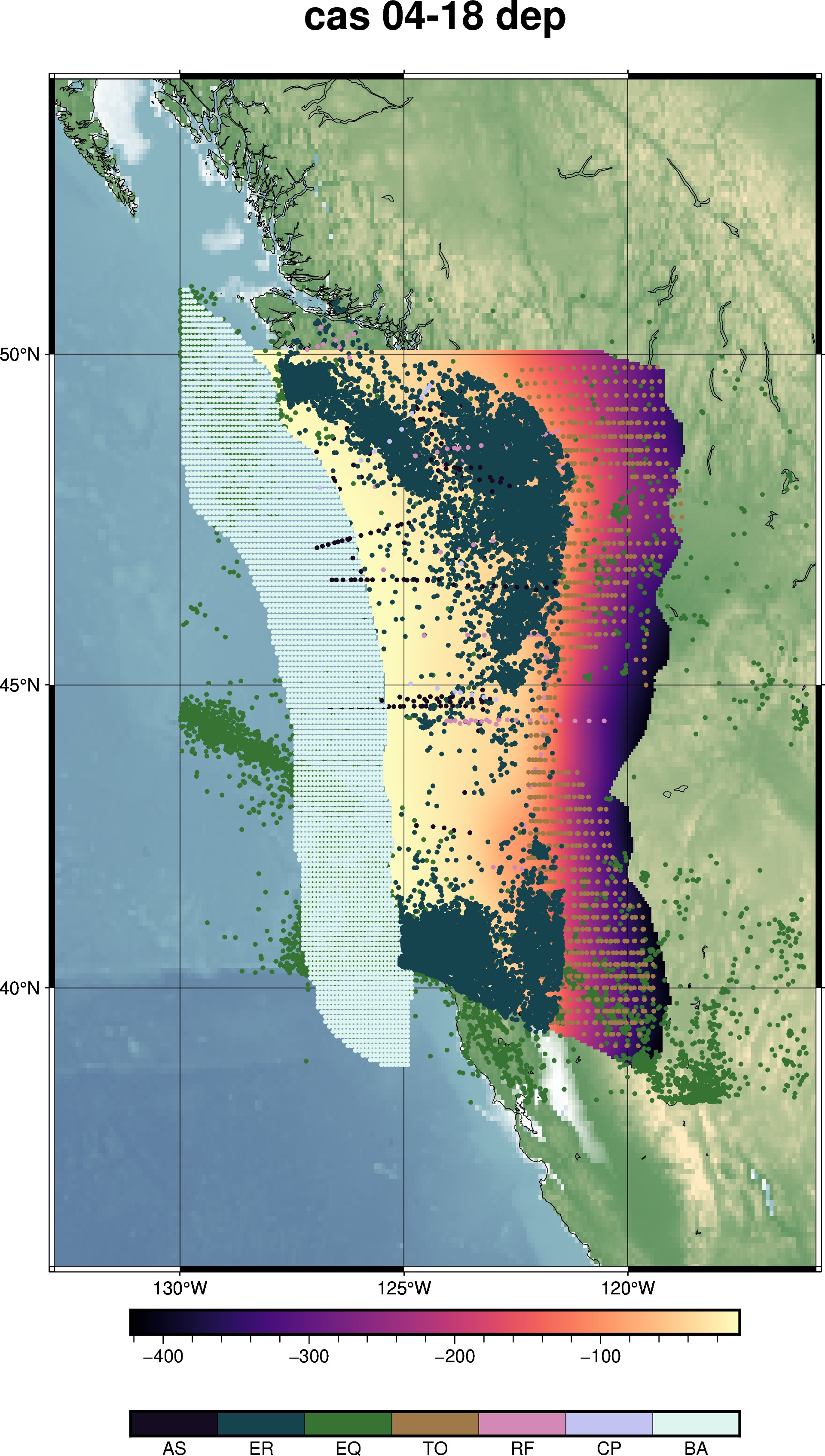
Cascadia surface model plot with input data.