Making a Slab Model
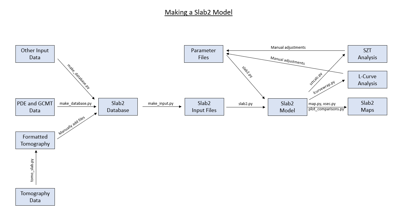
USGS Slab Models provides a highly customizable platform for generating slab geometry models with a variety of different input parameters. The outline below explains the process for producing your own slab model with the desired input data and parameters. The below figure shows the process for generating a new slab model.
Creating a Slab Model
To create a new slab model, you will need two things: a parameter file and an input file. A handful of input files are available in the repository, however if you wish to make a model with newer data, you will need to create a new input file first. For instructions on how to do so, visit the Making Input Files page.
To run the module, you will need to navigate to src/ and ensure the Python virtual environment is activated
using the command conda activate slab2env.
Next, input the command python slab2.py -p [path_to_parameter_file] -d [database MM-YY] -c [number of cores]
-l [slab model location]. Parameter files can be found in src/config/. Database refers to the directory containing
input files to use for the model, corresponging to the MM-YY date of the database used to create said input file.
Up to 4 cores may be used to speed up the model generation model, however this is optional and will default to
running on a single core if unspecified. The (surface or center) slab model location may also be specified when generating
a model. This argument is optional and will default to a slab surface model. Note that regions mue, sul, and ryu
are truncated by other slabs and require the depth grid of the truncating slab to be specified using the -u flag,
followed by the path to the depth grid file you would like to use (stored in the src/output/ folder).
Truncating slabs are as follows:
mue: truncated by car
sul: truncated by hal
phi: truncated by hal
ryu: truncated by kur
Parameter Files
USGS slab model parameter files can be found in the src/config/ folder, and contain the default parameters for running a slab model. These text files are used to assign values to parameter variables, which are then read during the execution of the slab.py module. To edit these parameters, the text files can be manually edited with a text editor. It is important to maintain the format of the parameter files when editing; only changing the values of the specified variables. Parameters which may be changed include:
inFile: defaults to “latest” unless using an input not stored in the input/input_files/ folder
use_box: option to use region boundaries specified in this parameter file. Else uses default values assigned to each slab region
latmin: lower region boundary latitude
latmax: upper region boundary latitude
lonmin: westmost region boundary longitude
lonmax: eastmost region boundary longitude
slab: 3-letter slab region code
grid: grid node spacing
radius1: long axis of search ellipsoid
radius2: short axis of search ellipsoid
sdr: shallow depth range to search for points above the slab guide
ddr: deep depth range to search for points below the slab guide
minunc: minimum uncertainty to use for earthquake data
mindip: low dip threshold for ellipsiod orientation
minstk: strike threshold for ellipsoid orientation
maxthickness: maximum slab thickness
seismo_thick: seismogenic zone thickness
dipthresh: high dip threshold for ellipsoid orientation
taper: depth over which to taper from no shift to full shift (km)
fracS: fraction of slab thickness to use for shift magnitude
T: tension for surface
node: grid node spacing for model output
filt: width of smoothing filter (degrees)
maxdist: distance-from-trench threshold for filtering
knot_no: default k0 value
kdeg: Kagan angle
rbfs: RBF smoothing factor
Note
Some parameters for certain models are automatically overwritten by code in slab2.py, slab2_functions.py, and loops.py.
To determine optimal parameters for a certain slab region, refer to the steps below.
Determining Shift Magnitude
The shift magnitude parameter is one of the more influential parameters used in generating a slab model. The shift magnitude is used to account for the difference between interslab and intraslab data, starting at the base of the seismogenic zone. It essentially shifts intraslab events to the slab interface. The optimal shift magnitude can be found by comparing the width of the event distribution with the inferred slab thickness at each node. Using the age of the oceanic lithosphere at the slab trench from Muller et al. (2008a) and the thermal boundary layer approximation from Turcotte and Schubert. (2002a), the total lithospheric thickness can be determined. More details for this method are explained in the supporting information for Hayes et al. (2018a). A percentage of this lithospheric thickness, fracshift is then used as the total shift magnitude. The shift magnitude however is non-linear. The taper parameter specifies the distance over which to increase the shift magnitude from zero to the full shift amount (fracshift). Seafloor age data is stored in src/polygons/interp_age.3.2g.nc.
Running L-Curve for a Model
The L-Curve can be used to determine the best width for the gaussian smoothing filter. The L-Curve for a given slab model can
be calculated by navigating to src/ and running the command: python lcurvewrap.py -p [path_to_parameter_file] -f [path_to_output_file].
Small models (e.g. sul) will take on the order of minutes to run, while larger models (e.g. sam) will take on the order of hours. Once
finished, the optimal smoothing filter will be output in the terminal labelled “bestfilt.” This value should be used as the “filt” value
in the parameter file for the given slab (can be changed by manually editing the parameter text file). Further assessment of this pick
can be done by analyzing the plots saved to the output folder for the selected model. To further optimize the smoothing filter, generate
a new model with the new smoothing filter added to the parameter file used, and repeat this process iteratively until optimal smoothness
is acheived.
Calculating Seismogenic Zone Width
A default seismogenic zone depth value of 45 km for generating new slab models is used. If you wish to perform a more in depth analysis
on the seismogenic zone of a specific slab model, the sztcalc.py module can be used. To perform the analysis, first change to the src/
directory and activate the Python environment. Use the command: python sztcalc.py -i [inputfolder] -f [filelist] -l [origorcentl] -d
[origorcentd] -b [slaborev] -m [maxdepdiff] -x [maxdep] where:
inputfolder:folder containing input files (e.g. input/input_files/04-18)
filelist:folder containing output files for the target model (e.g. src/output/[slab]_slab2_[model date])
origorcentl:“o” or “c” indicating origin or CMT longitude and latitude to compare with the slab
origorcentd:“o” or “c” indicating origin or CMT depth to compare with the slab
slaborev:“e” or “s” indicating a distribution of event depths or slab depths
maxdepdiff:A depth filter to exclude points outside of in szt calculations
maxdep:A depth extent to cut distributions off at
With optional arguments including:
-s:specifies surface or center slab model type
-o:specifies region boundaries with [minlon, maxlon, minlat, maxlat]
-k:path to a clipping mask
Resulting Seismogenic Zone data and analysis will be saved to the output folder for the desired slab model. After user interpretation, results can be used to adjust parameters for making new slab models of that region. To adjust parameters, simply open the parameter text file and edit the value of the seismo_thick variable manually.