plot.plot_clip

plot_clip(clp, fig=None, region=None, show=False, savefile=None, projection="M15c")

Plots outline of a clipping mask.

Arguments:

• clp (pd.DataFrame or str): clipping mask

• fig (pygmt.Figure, optional): figure object to append features to. Defaults to None.

• region (list, optional): defines the region extent[xmin,xmax,ymin,ymax,zmin,zmax]. Defaults to None.

• show (bool, optional): displays the figure. Defaults to False.

• savefile (str, optional): file path to save figure to

• projection (str, optional): map projection to use. Defaults to “M15c”.

Returns:

None

Example

import plot
import pygmt
# load in the synthetic test model as a slab_model instance
model = plot.slab_model("../output/exp_slab2_04-18","surface") # synthetic test slab made with the 04-18 database
# initialize figure as pygmt.Figure
fig = pygmt.Figure()
# making a plot of the model depth
plot.plot(
    model.dep_grid, # specifies which grid object to plot
    fig=fig, # add this plot to the existing figure
    contours=True, # add contour lines to the plot
    basemap=True, # add basemap to the plot
    nan_transparent=True, # removing nan values to make basemap visible
    title="exp slab model with 04-18 database", # adding a title to the plot
    dtype="depth", # specifying the datatype for labeling the colorbar
    region=model.region, # specifying the region boundaries to use
    show=False, # do not display the figure
)
# plotting the clipping mask on top of the model depth plot
plot.plot_clip(
    model.clp, # using the clipping mask associated with the previously defined model
    fig=fig, # add this plot to the existing figure
    region=model.region, # specify the region boundaries
    show=True, # display the figure now that all features have been added
    savefile="output/exp_slab2_04-18_depth_with_clip.jpg", # saving the figure to a jpeg file
)

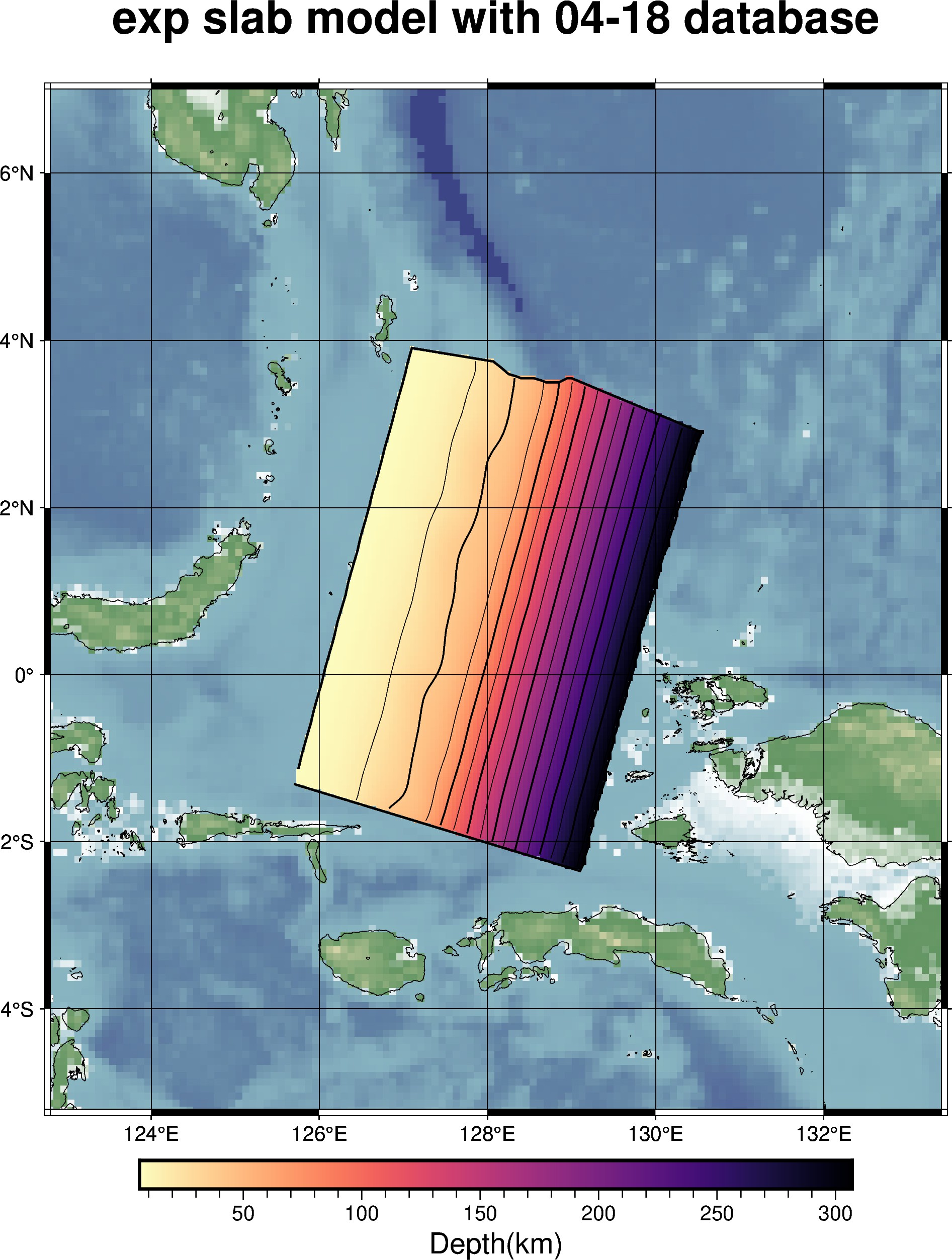
Output of example shown above