plot.plot_inputs

plot_inputs(data, fig=None, region=None, etype=None, show=False, savefile=None, projection="M15c")

Plots input data as a 2D scatter plot.

Arguments:

• data (pd.DataFrame or str): dataset of input data

• fig (pygmt.Figure, optional): figure object to append features to. Defaults to None.

• region (list, optional): specifies the region to use for plotting. Defaults to None.

• etype (list, optional): specifies type(s) of input data to plot. Defaults to None.

• show (bool, optional): show figure. Defaults to False.

• savefile (str, optional): file to save figure to

• projection (str, optional): map projection to use. Defaults to ‘M15c’.

Returns:

None

Example

import plot
import pygmt
# load in the synthetic test model as a slab_model instance
model = plot.slab_model("../output/exp_slab2_04-18","surface") # synthetic test slab made with the 04-18 database
# initialize figure as pygmt.Figure
fig = pygmt.Figure()
# making a plot of the model depth
plot.plot(
    model.dep_grid, # specifies which grid object to plot
    fig=fig, # add this plot to the existing figure
    basemap=True, # add basemap to the plot
    nan_transparent=True, # removing nan values to make basemap visible
    title="exp slab model with 04-18 database", # adding a title to the plot
    dtype="depth", # specifying the datatype for labeling the colorbar
    region=model.region, # specifying the region boundaries to use
    show=False, # do not display the figure
)
# overlaying the model inputs
plot.plot_inputs(
    model.input, # specify the input data to plot
    fig=fig, # add this plot to the existing figure
    region=model.region, # specify the region boundaries
    etype="EQ", # specify the data type to constrain dataset to
    show=True, # display the figure
    savefile="output/exp_slab2_04-18_depth_with_EQ.jpg" # save figure to jpeg file
)

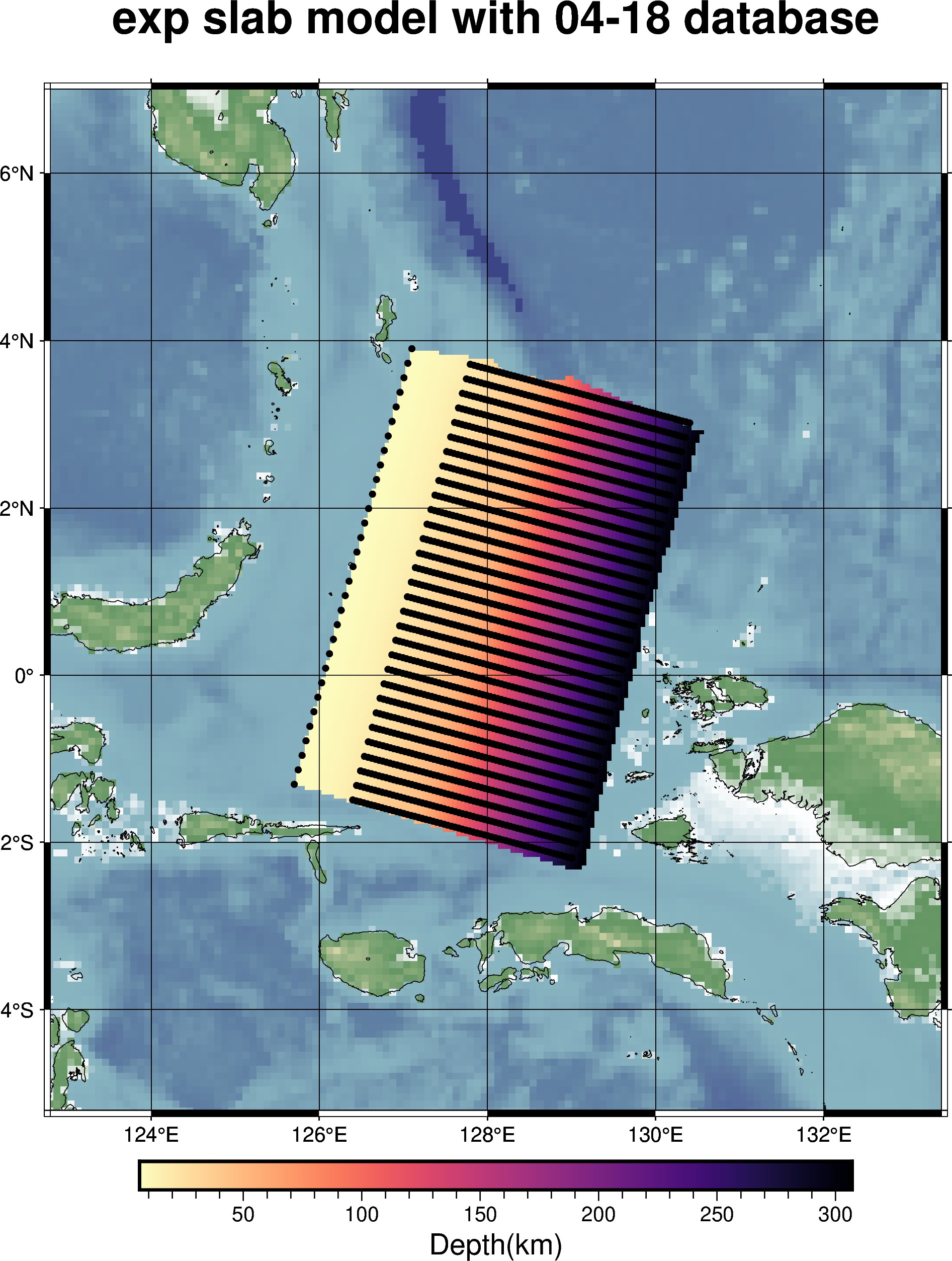
Output of example shown above