A Simple Introduction
This tutorial is meant to demonstrate the basics of how one would use gmprocess in an interactive python session and is meant for new users. For this tutorial, we will start by reading in some example data files with different formats.
Reading in data
First, we will create a list of the file names
from gmprocess.utils.constants import DATA_DIR

data_path = DATA_DIR / "demo" / "ci38457511" / "raw"
data_files = list(data_path.glob("*"))
for data_file in data_files:
    print(data_file)
/builds/ghsc/esi/groundmotion-processing/venv/lib/python3.12/site-packages/gmprocess/data/demo/ci38457511/raw/CICCC.RAW
/builds/ghsc/esi/groundmotion-processing/venv/lib/python3.12/site-packages/gmprocess/data/demo/ci38457511/raw/CICLC.v1
/builds/ghsc/esi/groundmotion-processing/venv/lib/python3.12/site-packages/gmprocess/data/demo/ci38457511/raw/CITOW2.RAW
Now we will read in one of the data files using gmprocess
from gmprocess.io.read import read_data

test = read_data(data_files[0])
Note that the warnings are because these data files do not report station elevation and in this case we put in a default value of zero.
The read_data function returns a list, but in this case it only has one element
print(f"{type(test)=}")
print(f"{len(test)=}")
type(test)=<class 'list'>
len(test)=1
And the element of the list is a StationStream object with three StationTraces in it
print(test[0])
3 StationTrace(s) in StationStream (passed):
CI.CCC.--.HN2 | 2019-07-06T03:19:37.000000Z - 2019-07-06T03:25:31.290000Z | 100.0 Hz, 35430 samples (passed)
CI.CCC.--.HN1 | 2019-07-06T03:19:37.000000Z - 2019-07-06T03:25:31.010000Z | 100.0 Hz, 35402 samples (passed)
CI.CCC.--.HNZ | 2019-07-06T03:19:37.000000Z - 2019-07-06T03:25:31.050000Z | 100.0 Hz, 35406 samples (passed)
Please see the Core gmprocess Objects section of the manual for more details about the StationStream and StationTraces objects. But put simply:
A StationStream is a container for one or more StationTrace objects.
A StationTrace is a container for a single channel waveform.
StationStream and StationTrace are the gmprocess analogs of ObsPy’s Stream and Trace objects.
A summary of the trace metadata is stored in the stats attribute just like ObsPy traces:
print(test[0][0].stats)
         network: CI
         station: CCC
        location: --
         channel: HN2
       starttime: 2019-07-06T03:19:37.000000Z
         endtime: 2019-07-06T03:25:31.290000Z
   sampling_rate: 100.0
           delta: 0.01
            npts: 35430
           calib: 1.0
     coordinates: AttribDict({'latitude': 35.525, 'longitude': -117.365, 'elevation': 0.0})
 format_specific: AttribDict({'fractional_unit': 1.0, 'sensor_sensitivity': 4989.676, 'time_sd': nan})
        standard: AttribDict({'units_type': 'acc', 'units': 'cm/s^2', 'horizontal_orientation': 90.0, 'vertical_orientation': nan, 'instrument_period': 0.005, 'instrument_damping': 0.7071, 'process_time': '2019-07-06T00:00:00Z', 'process_level': 'uncorrected physical units', 'comments': '', 'structure_type': '', 'instrument': 'Q330', 'sensor_serial_number': '4114', 'corner_frequency': nan, 'source': 'Southern California Seismic Network, California Institute of Technology (Caltech)', 'source_format': 'dmg', 'station_name': 'China Lake NWC, Christmas Canyon Rd.', 'instrument_sensitivity': nan, 'volts_to_counts': nan, 'source_file': 'CICCC.RAW', 'structure_cosmos_code': 999})
It would be convenient for us to make a list that consists of the three different stations that we originally read in. And we can do that with
streams = []
for data_file in data_files:
    streams.append(read_data(data_file)[0])
Note that the [0] at the end of the last line is to select the first and only element of the list returned by the read_data function.
Important
It is worth emphasizing that an important feature of gmprocess is that although these data were stored in different formats, once they are read into gmprocess the data is now in a consistent format and the user doesn’t have to worry about the peculiarities of the many different ground motion data formats that are commonly encountered.
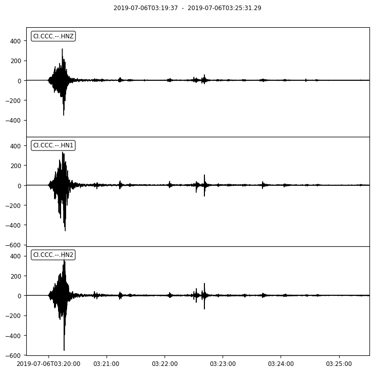
To plot the data from one of the StationStreams
Processing
One of the first things we typically want to do with records is to detrend. This is easily done with ObsPy functions
for stream in streams:
    stream.detrend(type="linear")
    stream.detrend(type="constant")
Typically, we would also remove the instrument response, but that has already been done for these records.
This is documented in the process_level in the trace stats.
We will print it here for the first trace in the first stream:
print(streams[0][0].stats.standard.process_level)
print(streams[0][0].stats.standard.units)
print(streams[0][0].stats.standard.units_type)
uncorrected physical units
cm/s^2
acc
Note that if the instrument response had not been removed, process_level would be “raw counts”.
We also show the units and units_type attributes.
If the instrument response were not removed, then units would be “counts”;
units_type indicates if the units are for acceleration, velocity, or displacement.
In order to proceed, we will want to split the records into the noise and signal windows. This relies on computing the P-wave travel time and so the earthquake associated with the ground motions is required. The easiest way to get this is from the USGS event id:
from gmprocess.core.scalar_event import ScalarEvent
from gmprocess.utils.download_utils import download_comcat_event

event_id = "ci38457511"
event_info = download_comcat_event(event_id)
event = ScalarEvent.from_json(event_info)
print(event)
Event:	2019-07-06T03:19:53.040000Z | +35.770, -117.599 | 7.1  mw

	 resource_id: ResourceIdentifier(id="ci38457511")
	        ---------
	     origins: 1 Elements
	  magnitudes: 1 Elements
We can now call the signal_split processing step:
from gmprocess.waveform_processing.windows import signal_split

for stream in streams:
    stream = signal_split(stream, event)
This provides a new parameter to each trace called signal_split
print(streams[0][0].get_parameter("signal_split"))
{'split_time': UTCDateTime(2019, 7, 6, 3, 19, 57, 347864), 'method': 'p_arrival', 'picker_type': 'median(travel_time, ar, baer, power, kalkan)'}
And we also want to similarly add the signal end time:
from gmprocess.waveform_processing.windows import signal_end

for stream in streams:
    stream = signal_end(
        stream,
        event.time,
        event.longitude,
        event.latitude,
        event.magnitude,
    )
Now we can compute the signal-to-noise ratio
from gmprocess.waveform_processing.snr import compute_snr, snr_check

for stream in streams:
    stream = compute_snr(stream, event)
    stream = snr_check(stream, event.magnitude)
And use the signal-to-noise ratio to compute the corner frequencies
from gmprocess.waveform_processing.corner_frequencies import get_corner_frequencies

for stream in streams:
    stream = get_corner_frequencies(stream, event)
Note that the selected corner frequencies can be accessed as
print(streams[0][0].get_parameter("corner_frequencies"))
{'type': 'snr', 'highpass': 0.02665449864674412, 'lowpass': 49.99999999999999}
Then we can cut, taper, apply the corner frequencies, and detrend based on the mean of the pre-event noise and a baseline correction
from gmprocess.waveform_processing.windows import cut
from gmprocess.waveform_processing.taper import taper
from gmprocess.waveform_processing.filtering import highpass_filter, lowpass_filter
from gmprocess.waveform_processing.detrend import detrend

for stream in streams:
    stream = cut(stream)
    stream = taper(stream)
    stream = highpass_filter(stream, event)
    stream = lowpass_filter(stream, event)
    stream = detrend(stream, detrending_method="pre")
    stream = detrend(stream, detrending_method="baseline_sixth_order")
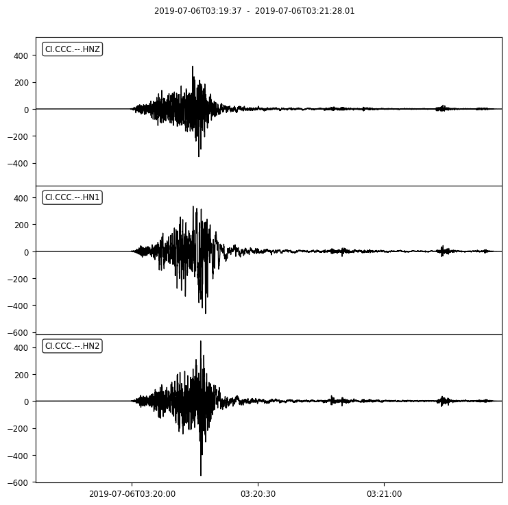
And we can plot the processed waveforms and compare to the unprocessed waveforms above
Computing metrics
At this point, computing waveform metrics is relatively easy using the WaveformMetricCollection class
from gmprocess.utils.config import get_config
from gmprocess.metrics.waveform_metric_collection import WaveformMetricCollection

config = get_config()
wmc = WaveformMetricCollection.from_streams(streams, event, config)
print(wmc)
WaveformMetricCollection: 3 stations
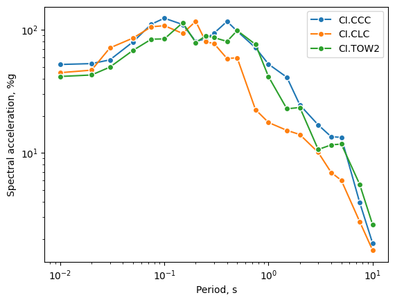
In order to re-organize the data a bit to make it more convenient to plot the RotD50 response spectra, it is useful to convert the WaveformMetricCollection to a Pandas dataframe:
sa_rotd_dfs = []
for wml in wmc.waveform_metrics:
    tmp_df = wml.select("PSA").to_df()
    tmp_df = tmp_df.loc[tmp_df["IMC"] == "RotD(percentile=50.0)"]
    sa_rotd_dfs.append(tmp_df)
And now we can plot the RotD50 response spectra, with a little bit of trouble to get the period out of the intensity metric type (IMT) column
import matplotlib.pyplot as plt

def imt_to_period(imt):
    return float(imt.split(",")[0].split("=")[1])

def plot_sa(ax, df, sta):
    per = [imt_to_period(imt) for imt in df["IMT"]]
    ax.loglog(per, df["Result"], label=sta, marker="o", mec="white")

codes = [f"{st[0].stats.network}.{st[0].stats.station}" for st in streams]

fig, ax = plt.subplots()
for tmp_df, code in zip(sa_rotd_dfs, codes):
    plot_sa(ax, tmp_df, code)
ax.set_xlabel("Period, s")
ax.set_ylabel("Spectral acceleration, %g")
ax.legend();


