Linear Mixed Effects Regressions

After assembling a ground motion database with gmprocess, linear mixed effects models can be used to analyze trends in the data. In this tutorial, we will read in some sample ground motion data, compute residuals relative to a ground motion model, and perform a linear, mixed effects regression to estimate the between- and within-event terms.

First, we import the necessary packages:

import numpy as np
import pandas as pd
import matplotlib.pyplot as plt
import statsmodels.formula.api as smf

from openquake.hazardlib import valid
from openquake.hazardlib.imt import SA
from openquake.hazardlib.contexts import simple_cmaker
from gmprocess.utils.constants import DATA_DIR

This tutorial uses the statsmodels package to create a mixed effects regression from spectral accelerations output from gmprocess.

We are using a ground motion dataset of earthquakes from the 2019 Ridgecrest, California Earthquake Sequence.

# Path to example data
data_path = DATA_DIR / "lme" / "SA_rotd50.0_2020.03.31.csv"
df = pd.read_csv(data_path)

We will use the ASK14 ground motion model (GMM) and spectral acceleration for an oscillator period of 1.0 seconds.

gsim = valid.gsim('''[AbrahamsonEtAl2014]''')
imt = SA(1.0)

To evaluate the GMM, we must make some simple assumptions regarding the rupture properties (dip, rake, width, ztor) and site properties (Vs30, Z1).

predicted_data = []

cmaker = simple_cmaker([gsim], [str(imt)], mags=["%2.f" % mag for mag in df.EarthquakeMagnitude])
n = df.shape[0]
ctx = cmaker.new_ctx(n)
ctx["mag"] = df.EarthquakeMagnitude
ctx["dip"] = 90.0
ctx["rake"] = 0.0
ctx["width"] = 10**(-0.76 + 0.27 * df.EarthquakeMagnitude)
ctx["ztor"] = df.EarthquakeDepth
ctx["vs30"] = 760.0
ctx["vs30measured"] = False
ctx["rrup"] = df.RuptureDistance
ctx["rjb"] = df.JoynerBooreDistance
ctx["z1pt0"] = 48.0
ctx["rx"] = -1
ctx["ry0"] = -1

# Evaluate the GMM.
mean = cmaker.get_mean_stds([ctx])[0][0][0]
# Convert from ln(g) to %g
predicted_data = 100.0 * np.exp(mean)

Now add the model residuals to the dataframe:

resid_col = 'SA_1_ASK14_residuals'
df[resid_col] = np.log(df['SA(1.000)']) - np.log(predicted_data)

For the linear mixed effects regression, we use the ‘EarthquakeId’ column to group the data by event to compute the between-event and within-event terms.

mdf = smf.mixedlm('%s ~ 1' % resid_col, df, groups=df['EarthquakeId']).fit()
print(mdf.summary())

Mixed Linear Model Regression Results
==================================================================
Model:            MixedLM Dependent Variable: SA_1_ASK14_residuals
No. Observations: 22375   Method:             REML                
No. Groups:       131     Scale:              0.6680              
Min. group size:  1       Log-Likelihood:     -27457.3530         
Max. group size:  767     Converged:          Yes                 
Mean group size:  170.8                                           
---------------------------------------------------------------------
             Coef.    Std.Err.      z       P>|z|    [0.025    0.975]
---------------------------------------------------------------------
Intercept    0.828       0.046    17.899    0.000     0.737     0.919
Group Var    0.245       0.045                                       
==================================================================

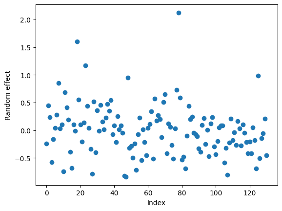
The model yields a bias (intercept) of 0.828. We can also look at the between-event terms with in the random_effects attribute, which is a dictionary with keys corresponding to the random effect grouping.

re_array = [float(re.iloc[0]) for group, re in mdf.random_effects.items()]
plt.plot(re_array, 'o')
plt.xlabel('Index')
plt.ylabel('Random effect');

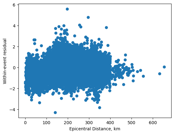
and the within-event residuals

plt.plot(df['EpicentralDistance'], mdf.resid, 'o')
plt.xlabel('Epicentral Distance, km')
plt.ylabel('Within-event residual');

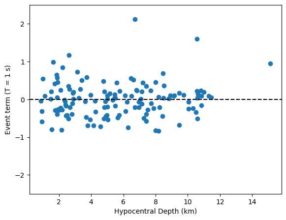
It is useful to merge the random effect terms with the original dataframe to look at the between-event terms as a function of other parameters, such as hypocentral depth.

btw_event_terms = pd.DataFrame(mdf.random_effects).T
df = df.merge(btw_event_terms, left_on='EarthquakeId', right_index=True)
df_events = df.drop_duplicates(subset=['EarthquakeId'])

fig = plt.figure()
axes = fig.add_axes([0.1, 0.1, 0.8, 0.8])
axes.scatter(df_events['EarthquakeDepth'], df_events['Group'])
axes.set_xlabel('Hypocentral Depth (km)')
axes.set_ylabel('Event term (T = 1 s)')
axes.axhline(0, ls='--', c='k')
axes.set_ylim(-2.5, 2.5);