Graphical User Interface (GUI) to aid human review of processed-ground-motions

Authors

Maria E. Ramos-Sepulveda, Scott J. Brandenberg, Tristan Buckreis, Meibai Li, Shako Ahmed, and Jonathan P. Stewart

The UCLA geotechnical group prepared a graphical user interface (GUI) to facilitate a human review of records processed by gmprocess. The algorithms utilized by gmprocess to accept/reject, window, and filter records work well most of the time, but cannot account for all possible issues that might arise. For this reason, reviewing the processed records is prudent. The purpose of this GUI is to facilitate rapid review. Acceleration and displacement time series, as well as response spectra can be visually inspected to find any potential errors. The GUI utilizes Jupyter and allows the user to load an HDF5 file output from gmprocess, interact with the data by accepting or rejecting records, and adjusting high-pass and low-pass filter parameters. In the example below we describe the procedure to run and interact with the GUI.

Requirements

• A workspace.h5 file produced by gmprocess through the “process_waveforms” step. For example gmrecords --eventid nc73291880 download, gmrecords assemble and gmrecords process_waveforms must be run before going through this review step.

• The Python script named HumanReviewGUI.py that contains the class variable and function defintions that will be called by a Jupyter Notebook.

• A Jupyter Notebook that instantiates the HumanReviewGUI class.

• gmprocess

• obspy

• ipywidgets

• pandas

• numpy

• matplotlib

• ucla_geotech_tools.response_spectrum

• json

• prov

• ipympl

Jupyter notebook

Creating the GUI requires only three lines of code, shown below. Older versions of Jupyter might require %matplotlib notebook instead of %matplotlib widget. Running these three lines should produce plots like the ones shown in the sections that follow.

%matplotlib widget
import gmprocess.gui.gui_ucla.HumanReviewGUI as HRG
GUI = HRG.HumanReviewGUI()

Plots description

The interface is shown in Figure 1, and consists of a control panel and four plots. The control panel contains a field where users input the filename and load the HDF5 file. The progress bar on top displays how many records have been loaded. Once the loading is done, the progress bar reflects how many records have been accepted. The toggle buttons next to the load button filter data by showing only data waveforms that have not been reviewed, those that have been accepted, and/or those that have been rejected. The third row of the control panel has buttons to browse to the previous or next record, along with a dropdown menu for selecting a specific record. Next to the right are the buttons for accepting or rejecting the record. A record should be accepted when the user considers it to have been processed correctly, and rejected when the user believes that the record should not be processed because it is too noisy or has other flaws. The bottom row of the control panel contains the name of the user who processed the record, the earthquake magnitude, and the epicentral distance. Users can also set the high-pass and low-pass corner frequencies (fchp and fclp respectively), and uncheck a box to control whether the fclp is not applied at all. The filters utilize the same order and filter type as specified by the user in gmprocess and are not configurable in the GUI. We found that these options do not require adjustment after processing in gmprocess.

The orange traces depict the unfiltered record. In this context, “unfiltered” refers to the trace that has not gone through the Butterworth filter, but is trimmed, demeaned and tapered. The blue trace (“filtered GUI”) is filtered using the apply_filter function inside the python script and it will change if any of the corner frequencies are modified. The blue time series includes the minimum between 60 seconds of noise and the maximum noise length of a record while the traces called from gmprocess have 2 seconds (default in config file). The translucent red (“filtered gmprocess”) is the record filtered inside gmprocess. This trace will not change if the corner frequencies are modified. The purpose of including both filtered traces (blue and red) is so the user can compare any improvements done in the GUI. The red trace was set to translucent to aid the visual comparison. As a result of superimposing the red over the blue, this trace will seem purple whenever “filtered GUI” overlaps “filtered gmprocess”. The smoothed noise spectrum is shown in green and only for the Fourier transform spectra. The black dotted line is the theoretical acceleration decay at low frequency according to the $f^2$ model (Brune 1970; Boore and Bommer 2005), the user can use it as reference. The dashed-black lines depict corner frequencies in the Fourier transform spectra and the highest-usable period (factor of 0.8) in the response spectra. The grey solid and dashed lines are the signal-to-noise ratio (SNR) and SNR threshold, respectively. The ordinates on the the Fourier transform spectra are not meant to be used to read the SNR, the idea is to evaluate the SNR with respect to the SNR threshold, signal, and noise traces.

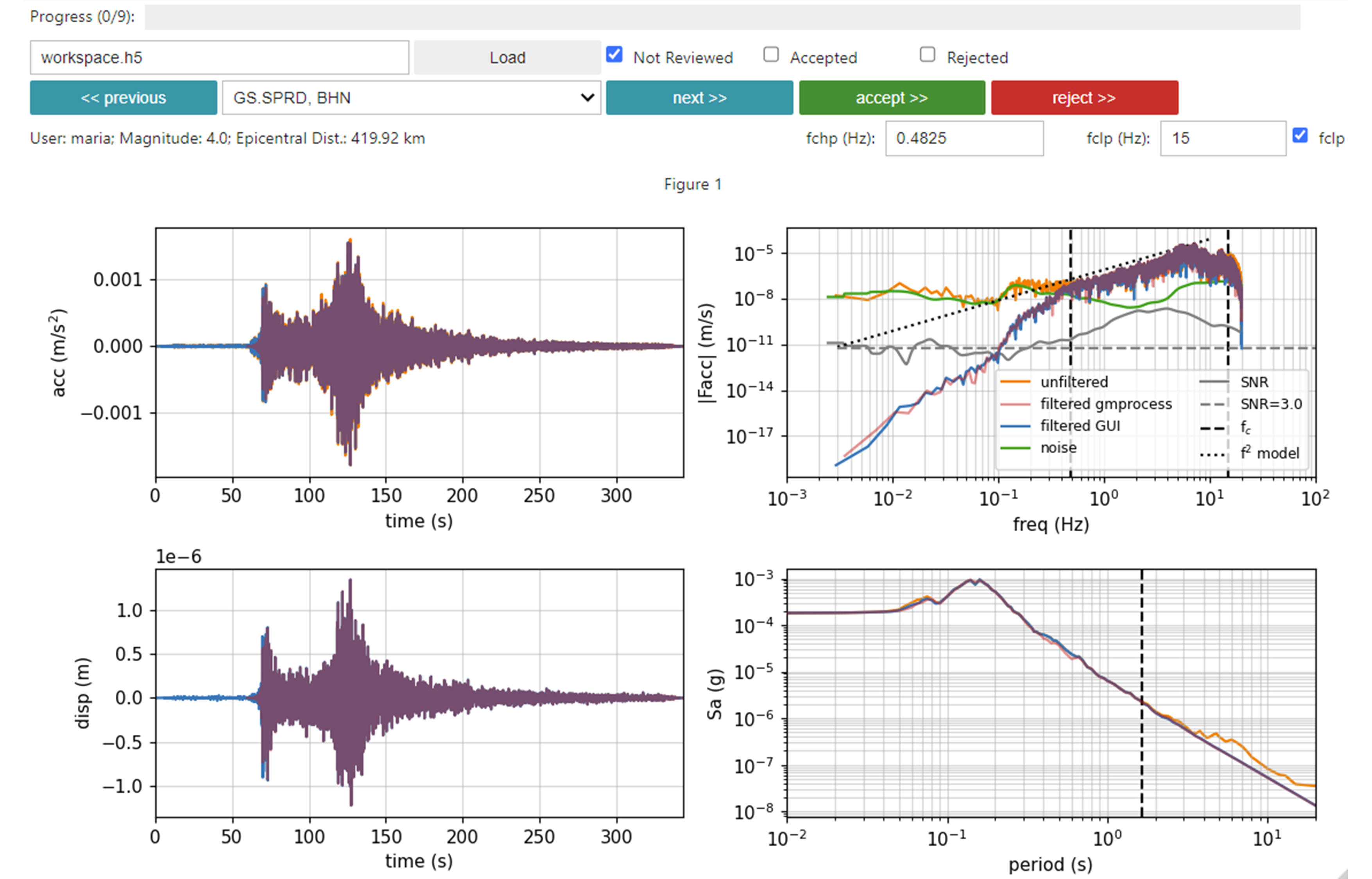
Figure 1: Interface of Graphic User Interface for human review

Procedure

Changes implemented in the GUI are recorded in the HDF5 file through an auxiliary_data folder named review. In the review section you can find which records were accepted or rejected and the corresponding corner frequency values. To integrate these changes into the provenance and update the waveforms, the user needs to run gmrecords process -r. The changes in the auxiliary_data folder will then be reflected in the provenance directory of the .h5 file.

The processing steps are listed below:

• Load workspace.h5

• Evaluate acceleration, displacement, amplitude and response plots.

• Increase values of fchp if necessary.

• Change and/or remove value of fclp if necessary.

• Accept or reject the record accordingly. The GUI will automatically proceed to the next trace.

• Run gmrecords process -r to overwrite the traces objects in the workspace.h5.

Changes in high-pass corner frequencies

The most common modification is an adjustment to the fchp. The automated selection of fchp is done using the auto_fchp package inside gmprocess, which fits a 6th order polynomial to the displacement trace and adjusts the fchp until the amplitude of the polynomial fit is a specified fraction of the amplitude of the displacement trace. Sometimes, the automated fchp value is not high enough to discard lingering long period noise (which can be observed as a wobbly displacement trace, shown in Figure 2). In this case, the fchp was increased to 0.19 Hz to render a displacement trace that is stable prior to the p-wave arrival, as shown in Figure 3.

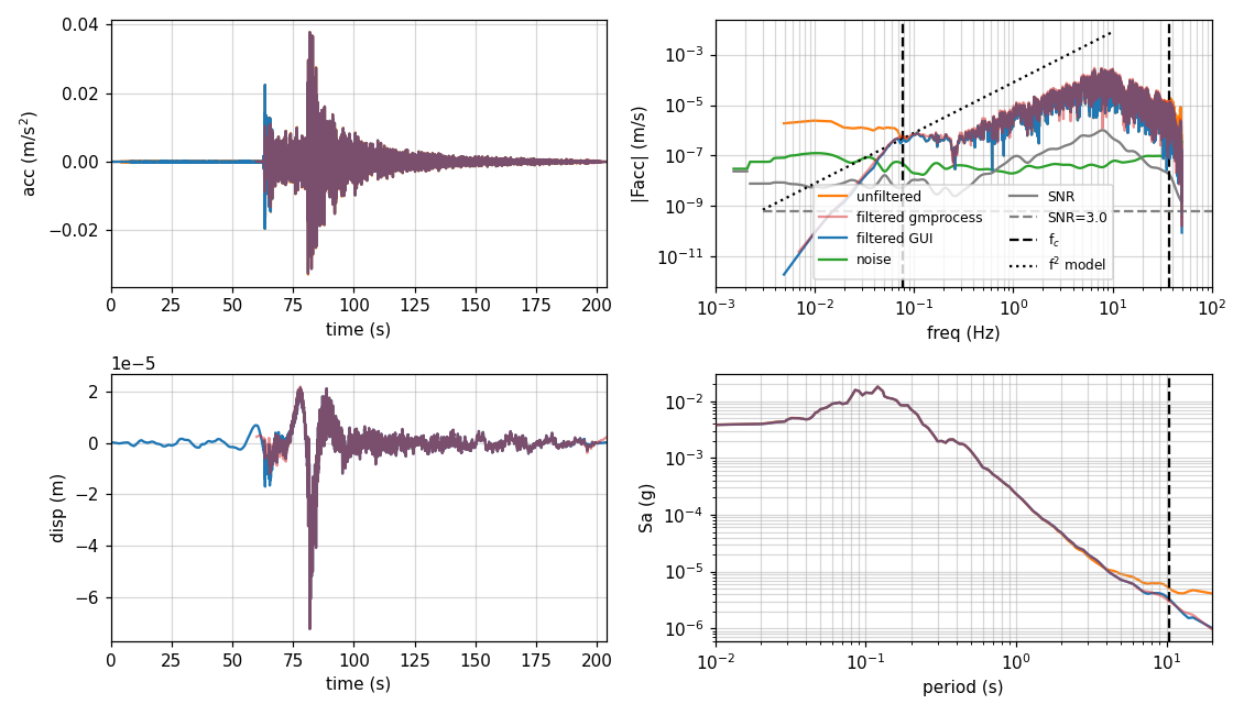
Figure 2: Example trace with an automated selected fchp resulting in an irregular displacement time series

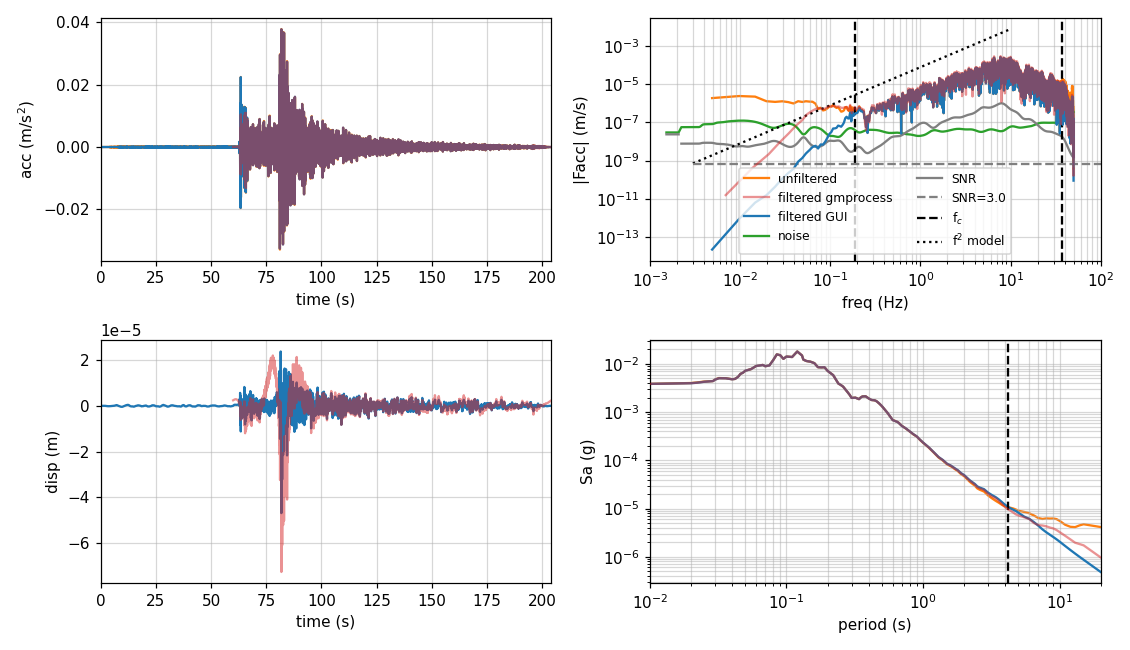
Figure 3: Example trace shown in Figure 2 with a modified fchp resulting in a regular displacement time series

Changes in low-pass corner frequencies

Depending on how the user configured their gmprocess, the fclp could be applied every time or never. In the GUI, by default, fclp is applied to the blue trace (“filtered GUI”). The value shown in the header of the plots is the fclp selected by gmprocess which is chosen to be the minimum between $0.7*Nyquist$ frequency and the highest frequency where SNR undergoes certain threshold. High amplitude short period noise could be reflected as an irregular peak in the response spectrum at short periods (Figure 4). The noise can be excluded from the trace by checking the box to the right and applying an fclp of the same value (Figure 5). In this case a low-pass filter at 14.6 Hz stabilized the short-period portion of the response spectrum.

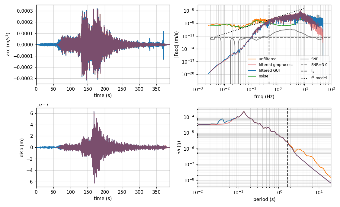
Figure 4: Example trace without fclp resulting in an irregular response spectra shape

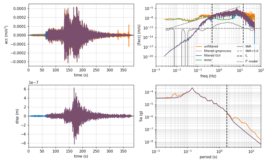
Figure 5: Example trace shown in Figure 4 with fclp resulting in a flat response spectra at short periods

Example of rejected record

Some records contaminated with significant noise might pass the “failing criteria” of gmprocess. We believe this may be the result of randomness in the pre-event noise window. Usually, these records are easy to spot in the acceleration time series. An example is shown in Figure 6. Although the earthquake trace is visible above the noise level, we consider this record to be too noisy and opted to reject it.

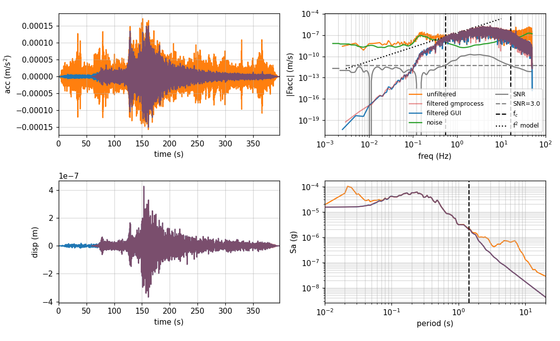
Figure 6: Example trace with significant noise that should be rejected

Limitations

1. Gmprocess might miscompute the location of the p-wave arrival or the coda. None of those issues could be further improved using the GUI.

2. The GUI will not update the provenance folder in the workspace.h5. If the user wants to pass this information from the auxiliary_data folder to the provenance folder and recompute the waveforms, the user needs to run gmrecords process -r.

3. The GUI will convert the units of unprocessed traces into $m/s^2$ if the raw data is in g units or in a mseed format. Otherwise, the traces in the plots will be offset and the user will have to go to the python code and apply the corresponding conversion.