Raster Factories Tutorial

This tutorial shows how to use the Raster class to load and build raster datasets from different data sources.

Introduction

There are many ways to acquire raster datasets when running hazard assessments. For example, a dataset may be loaded from a local file or web URL, or alternatively produced by performing computations on a numpy array. In other cases, you may want to rasterize a non-raster dataset - for example, converting a collection of Polygon features to a Raster representation.

To accommodate these diverse cases, the Raster class provides factory methods that create Raster objects for different data sources. Factories are the recommended way to create Raster objects, and they follow the naming convention from_<source>, where <source> indicates a particular type of data source. Commonly used factories include:

• from_file: Loads a raster from the local filesystem

• from_url: Loads a raster from a web URL

• from_array: Builds a Raster from a numpy array

• from_points: Builds a raster from a collection of Point features

• from_polygons: Builds a raster from a collection of Polygon features

and this tutorial will examine each of these commands.

Prerequisites

Install pfdf

To run this tutorial, you must have installed pfdf 3+ with tutorial resources in your Jupyter kernel. The following line checks this is the case:

import check_installation

pfdf and tutorial resources are installed

Imports

We’ll next import the Raster class from pfdf. We’ll also use numpy to create some example datasets, pathlib.Path to work with saved files, and the plot module to visualize datasets.

from pfdf.raster import Raster
import numpy as np
from pathlib import Path
from tools import plot

Example Files

Finally, we’ll save an example file to use in the tutorial. The example mimics a boolean raster mask that has been saved to file.

from tools import examples
examples.build_mask()

Built example raster mask

Raster.from_file

You can use the Raster.from_file command to return a Raster object for a dataset saved to the local filesystem. For example:

Raster.from_file('data/dnbr.tif')

Raster:
    Shape: (1280, 1587)
    Dtype: int16
    NoData: -32768
    CRS("NAD83 / UTM zone 11N")
    Transform(dx=10.0, dy=-10.0, left=408022.12009999994, top=3789055.5413000006, crs="NAD83 / UTM zone 11N")
    BoundingBox(left=408022.12009999994, bottom=3776255.5413000006, right=423892.12009999994, top=3789055.5413000006, crs="NAD83 / UTM zone 11N")

Inspecting our example dataset, we find the Raster holds the full 1280 x 1587 pixel data grid, which spans 15870 meters along the X axis, and 12800 meters along the Y axis.

The from_file command includes a variety of options, which you can read about in the API. One commonly used option is the bounds input, which lets you specify a bounding box in which to read data. This can be useful when your area-of-interest is much smaller than the saved raster dataset, and you want to limit the amount of data read into memory. The most common workflow is to use a second Raster object (often for a buffered fire perimeter) to define the bounding box.

For example, let’s make a mock fire perimeter that spans the top left quadrant of our dNBR raster. (You don’t need to understand the from_array command just yet - we’ll discuss it later in this tutorial):

perimeter = Raster.from_array(
    True, bounds={'left': 408022.1201, 'bottom': 3782655.5413, 'right': 415957.1201, 'top': 3789055.5413, 'crs': 26911}
)
print(perimeter.bounds)

BoundingBox(left=408022.1201, bottom=3782655.5413, right=415957.1201, top=3789055.5413, crs="NAD83 / UTM zone 11N")

We can now use this second Raster object to only load data from the top-left quadrant of the dNBR dataset:

Raster.from_file('data/dnbr.tif', bounds=perimeter)

Raster:
    Shape: (640, 794)
    Dtype: int16
    NoData: -32768
    CRS("NAD83 / UTM zone 11N")
    Transform(dx=10.0, dy=-10.0, left=408022.12009999994, top=3789055.5413000006, crs="NAD83 / UTM zone 11N")
    BoundingBox(left=408022.12009999994, bottom=3782655.5413000006, right=415962.12009999994, top=3789055.5413000006, crs="NAD83 / UTM zone 11N")

Inspecting the Raster, we find that command only loaded data for the 640 x 794 pixel grid in the top-left corner of the saved dataset. The bounding box is correspondingly smaller, and spans 7940 meters along the X axis, and 6400 meters along the Y axis.

Sometimes, you may want to load data in an explicit bounding box. In this case, you can provide the bounding box directly as input, without needing to load a second Raster object. The input bounding box may use any CRS, and will be reprojected if it does not match the CRS of the loaded raster. For example, let’s load the portion of the dNBR data spanning latitudes from 34.15 to 34.20 N, and longitudes from 117.85 to 117.95 W. We’ll define these coordinates in EPSG:4326 (also known as WGS-84):

bounds = {'left': -117.95, 'right': -117.85, 'bottom': 34.15, 'top': 34.20, 'crs': 4326}
Raster.from_file('data/dnbr.tif', bounds=bounds)

Raster:
    Shape: (562, 927)
    Dtype: int16
    NoData: -32768
    CRS("NAD83 / UTM zone 11N")
    Transform(dx=10.0, dy=-10.0, left=412422.12009999994, top=3784735.5413000006, crs="NAD83 / UTM zone 11N")
    BoundingBox(left=412422.12009999994, bottom=3779115.5413000006, right=421692.12009999994, top=3784735.5413000006, crs="NAD83 / UTM zone 11N")

Inspecting the raster, we find it holds the 562 x 927 data array located within the indicated coordinates.

Raster.from_url

You can use Raster.from_url to load a raster from a web URL. The command supports all the options of Raster.from_file, with some additional options for establishing web connections. We recommend using the bounds options with Raster.from_url whenever possible. Just like the from_file command, the bounds option instructs the command to only load data from the indicated bounding. This helps limit the total amount of data that needs to be transferred over an internet connection.

For example, the USGS distributes its 10 meter DEM product as a tiled dataset, with each tile spanning 1x1 degree of longitude and latitude. The tiles can be accessed via web URLs, but each tile requires ~400 MB of memory, which can take a while to download. Here, we’ll use the bounds option to download a subset of data from one of these tiles. Specifically, we’ll download DEM data near the town of Golden, Colorado:

bounds = {'left': -105.239773, 'right': -105.206539, 'bottom': 39.739556, 'top': 39.782944, 'crs': 4326}
url = 'https://prd-tnm.s3.amazonaws.com/StagedProducts/Elevation/13/TIFF/historical/n40w106/USGS_13_n40w106_20230602.tif'
raster = Raster.from_url(url, bounds=bounds)
print(raster)

Raster:
    Shape: (469, 359)
    Dtype: float32
    NoData: -999999.0
    CRS("NAD83")
    Transform(dx=9.25925927753796e-05, dy=-9.259259269220167e-05, left=-105.2398148142506, top=39.78296296356804, crs="NAD83")
    BoundingBox(left=-105.2398148142506, bottom=39.7395370375954, right=-105.20657407344423, top=39.78296296356804, crs="NAD83")

Inspecting the memory footprint of the loaded data, we find it uses ~673 KB, significantly less than the ~400 MB of the full DEM tile:

print(f'nbytes = {raster.nbytes}')

nbytes = 673484

One of the key connection options is the timeout parameter. This option specifies a maximum time to establish an initial connection with the URL server. (This is not the total download time, which can be much longer). By default, this is set to 10 seconds, but you might consider raising this time limit if you’re on a slow connection. For example, the following will allow 60 seconds to establish a server connection:

# Allows a full minute to establish a connection
raster = Raster.from_url(url, bounds=bounds, timeout=60)

Boolean Masks

Boolean raster masks are commonly used when working with pfdf. A raster mask is a raster dataset in which all the data values are 0/False or 1/True. These values are used to selectively choose pixels in an associated data raster of the same shape. For example, you might use a mask to indicate pixels that should be included/ignored in an analysis.

When working with numpy arrays, raster masks are best represented as arrays with a bool (boolean) dtype. However, many raster file formats do not support boolean data types, so instead save masks as the integers 1 and 0. This can cause problems, as numpy interprets integer indices differently from booleans.

As such, the from_file and from_url factories include a isbool option. Setting this option to True indicates that a saved raster represents a boolean mask, rather than an integer data array. When you use this option, the Raster object’s data array will have a bool dtype, and will be suitable for masking with numpy. We strongly recomend using this option whenever you load a saved raster mask.

For example, if we naively load our example mask, we find the output Raster has an integer dtype:

raster = Raster.from_file('examples/mask.tif')
print(raster.dtype)
print(raster.values)

int8
[[0 0 0 ... 0 0 0]
 [0 0 1 ... 0 1 0]
 [0 0 1 ... 1 0 0]
 ...
 [0 0 0 ... 1 1 0]
 [0 0 0 ... 1 0 0]
 [0 0 0 ... 0 0 0]]

But if we use the isbool option, then the Raster has the correct dtype and can be used for numpy indexing:

raster = Raster.from_file('examples/mask.tif', isbool=True)
print(raster.dtype)
print(raster.values)

bool
[[False False False ... False False False]
 [False False  True ... False  True False]
 [False False  True ...  True False False]
 ...
 [False False False ...  True  True False]
 [False False False ...  True False False]
 [False False False ... False False False]]

Raster.from_array

You can use the from_array factory to build a Raster from a numpy array or array-like object.

Spatial Metadata

Since numpy arrays do not include spatial metadata, a basic call to this factory will result in a Raster object without spatial metadata. For example:

values = np.arange(100).reshape(10,10)
Raster.from_array(values)

Raster:
    Shape: (10, 10)
    Dtype: int64
    NoData: -9223372036854775808
    CRS: None
    Transform: None
    BoundingBox: None

As such, the from_array factory includes a variety of options to specify this metadata. For example, you can use the crs option to specify a CRS, and either the transform or bounds option to specify either an affine transform or a bounding box:

Raster.from_array(values, crs=4326, bounds=[-117.95, 34.15, -117.85, 34.20])

Raster:
    Shape: (10, 10)
    Dtype: int64
    NoData: -9223372036854775808
    CRS("WGS 84")
    Transform(dx=0.010000000000000852, dy=-0.005000000000000426, left=-117.95, top=34.2, crs="WGS 84")
    BoundingBox(left=-117.95, bottom=34.15, right=-117.85, top=34.2, crs="WGS 84")

Note that you can only provide one of the transform or bounds options, as they actually provide the same information, albeit in different formats. In the example above, we did not provide a CRS for the bounding box, so the bounding box coordinates were interpreted in the input CRS (in this case EPSG:4326, which has units of degrees). However, if the bounding box also has a CRS, then the box will be reprojected to match the input CRS for the raster. For example:

bounds = {'left': 408022.1201, 'bottom': 3782655.5413, 'right': 415957.1201, 'top': 3789055.5413, 'crs': 26911}
Raster.from_array(values, crs=4326,  bounds=bounds)

Raster:
    Shape: (10, 10)
    Dtype: int64
    NoData: -9223372036854775808
    CRS("WGS 84")
    Transform(dx=0.008677698215561237, dy=-0.005838190366991824, left=-117.99877564871494, top=34.23920369335487, crs="WGS 84")
    BoundingBox(left=-117.99877564871494, bottom=34.18082178968495, right=-117.91199866655933, top=34.23920369335487, crs="WGS 84")

Alternatively, you can use the spatial option to set the spatial metadata equal to the spatial metadata of another Raster object. This can be useful when performing computations on a raster’s data grid. For example, lets do some math on our example raster’s data grid, and then convert the results to a Raster object:

template = Raster.from_file('data/dnbr.tif')
results = template.values * 1.2
Raster.from_array(results, spatial=template)

Raster:
    Shape: (1280, 1587)
    Dtype: float64
    NoData: nan
    CRS("NAD83 / UTM zone 11N")
    Transform(dx=10.0, dy=-10.0, left=408022.12009999994, top=3789055.5413000006, crs="NAD83 / UTM zone 11N")
    BoundingBox(left=408022.12009999994, bottom=3776255.5413000006, right=423892.12009999994, top=3789055.5413000006, crs="NAD83 / UTM zone 11N")

Inspecting the output, we find the new Raster object has the same CRS, transform, and bounding box as the template raster.

NoData Value

By default, from_array will attempt to determine a NoData value for the Raster from the array dtype. As follows:

dtype	Default Nodata
float	NaN
signed integers (int)	Most negative representable value
unsigned integers (uint)	Most positive representable value

Alternatively, you can use the nodata option to specify the NoData value explicitly. For example:

values = np.zeros((10,10), float)
default = Raster.from_array(values)
explicit = Raster.from_array(values, nodata=-9999)

print(default.nodata)
print(explicit.nodata)

nan
-9999.0

Raster.from_polygons

You can also use raster factories to rasterize vector feature datasets. We’ll begin with the from_polygons factory, which converts a Polygon/MultiPolygon feature collection to a raster. The command requires the path to a vector feature file as input. For example, the perimeter.geojson file from the hazard assessment tutorial is a Polygon collection:

raster = Raster.from_polygons('data/perimeter.geojson')
print(raster)

Raster:
    Shape: (680, 987)
    Dtype: bool
    NoData: False
    CRS("NAD83 / UTM zone 11N")
    Transform(dx=10.0, dy=-10.0, left=411022.12009999994, top=3786055.5413000006, crs="NAD83 / UTM zone 11N")
    BoundingBox(left=411022.12009999994, bottom=3779255.5413000006, right=420892.12009999994, top=3786055.5413000006, crs="NAD83 / UTM zone 11N")

Resolution

By default, the command rasterizes polygons to a 10 meter resolution, which is the recommended resolution for many of pfdf’s hazard models:

raster.resolution('meters')

(10.0, 10.0)

But you can use the resolution option to set a different resolution instead:

raster = Raster.from_polygons('data/perimeter.geojson', resolution=30, units='meters')
raster.resolution('meters')

(30.0, 30.0)

Data Fields

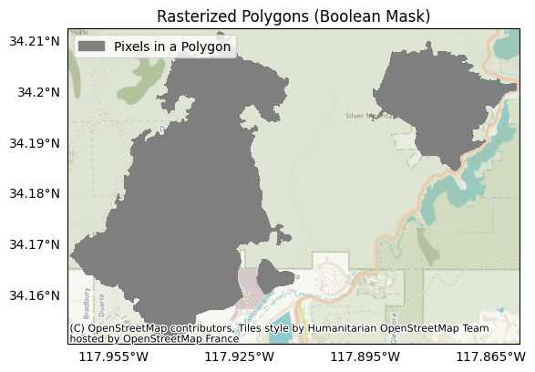
By default, from_polygons will build a boolean raster mask, where True pixels indicate locations within one of the polygons. However, you can use the field option to instead build the raster from one of the polygon data fields. In this case, pixels in a polygon will be set to the value for that polygon, and all other pixels are NoData.

For example, our example fire perimeter consists of several polygons, which are derived from the burn areas for the Reservoir and Fish fires. The dataset also includes a data field named my-data, which indicates which fire a polygon is associated with: a value of 1 indicates the Reservoir Fire, and 2 indicates the Fish fire. If we rasterize the dataset without specifying a data field, then the from_polygons command ignores the data field, and interprets the dataset as a boolean raster mask. Plotting the example, we find that raster pixels within the polygons are marked as True (dark grey), and pixels outside the squares are marked as False (white):

raster = Raster.from_polygons('data/perimeter.geojson')
plot.mask(raster, title='Rasterized Polygons (Boolean Mask)', legend='Pixels in a Polygon')

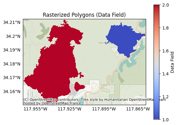
By contrast, if we rasterize the polygons from a data field, then the pixel values are determined by the data field for the associated polygon. For example, if we rasterize the example using the my-data field, then the pixels within the polygons are set to the associated field value, which in this case corresponds to the associated fire. Note that pixels outside of the polygons are set to NoData:

raster = Raster.from_polygons('data/perimeter.geojson', field='my-data')
plot.raster(raster, title='Rasterized Polygons (Data Field)', cmap='coolwarm', clabel='Data Field', show_basemap=True)

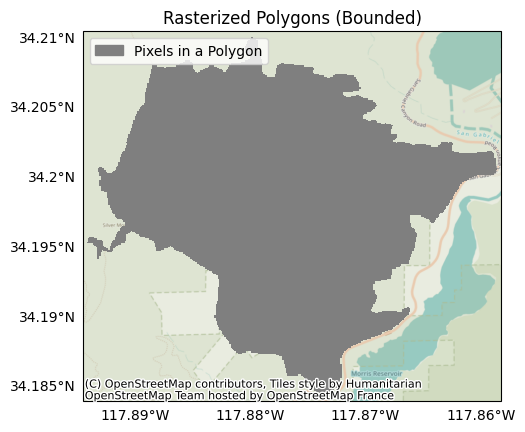
Bounding Box

It’s not uncommon to have a Polygon dataset that covers a much larger spatial area than your area of interest. When this is the case, rasterizing the entire polygon dataset can require an excessive amount of memory. Instead, use the bounds option to only rasterize the polygon features that intersect the given bounding box. As with the from_file factory, the most common workflow is to use a second Raster object as the bounding box. However, you can also provide the bounds explicitly if known.

For example, let’s use the bounds option to only rasterize the portion of the fire perimeter corresponding to the Reservoir Fire:

bounds = {'left': -117.894242, 'bottom': 34.1842093, 'right': -117.8585418, 'top': 34.2101890, 'crs': 4326}
raster = Raster.from_polygons('data/perimeter.geojson', bounds=bounds)
plot.mask(raster, title='Rasterized Polygons (Bounded)', legend='Pixels in a Polygon')

Raster.from_points

The syntax for the from_points factory is nearly identical to from_polygons, except that the file path should be for a Point/MultiPoint collection. When rasterizing points, raster pixels that contain a point will be set to True or the point’s data field, as appropriate.

Conclusion

In this tutorial, we’ve learned how to convert various types of datasets to Raster objects. We used:

• from_file to load a raster from the local file system

• from_url to load a raster from a web URL,

• from_array to add raster metadata to a numpy array

• from_polygons to rasterize a Polygon dataset, and

• from_points to rasterize a Point dataset.