Data Download Tutorial

This tutorial shows how to use the data subpackage to download hazard assessment datasets. Or skip to the end for a quick reference script.

Introduction

Hazard assessments require a variety of datasets. These include datasets used to delineate a stream segment network (such as fire perimeters and digital elevation models), and datasets used to implement hazard models (such as dNBRs and soil characteristics). Obtaining these datasets can represent a significant effort, requiring navigation of multiple data providers, each with their own systems and frameworks for distributing data.

As such, pfdf provides the data subpackage to help alleviate the difficulty of acquiring assessment datasets. This package provides routines to download various common datasets over the internet. These include:

• USGS digital elevation models (DEMs),

• NOAA Atlas 14 rainfall statistics,

• STATSGO KF-factors and soil thicknesses,

• LANDFIRE existing vegetation types (EVTs),

• Debris retainment feature locations, and

• Hydrologic unit (HU) boundaries and datasets.

In this tutorial we will use the data subpackage to acquire these datasets for the 2016 San Gabriel Fire Complex in California. Note that we will not be downloading the fire perimeter, burn severity, or dNBR datasets in this tutorial, as these datasets are typically provided by the user.

Important!

You are NOT required to use these datasets for your own assessments. The data subpackage is merely intended to facilitate working with certain commonly used datasets.

Suggesting Datasets

We welcome community suggestions of datasets to include in the data package. To suggest a new dataset, please contact the developers or the Landslides Hazards Program.

Prerequisites

Raster Tutorial

This tutorial assumes you are familiar with Raster objects and their metadata. Please read the Raster Intro Tutorial if you are not familiar with these concepts.

Install pfdf

To run this tutorial, you must have installed pfdf 3+ with tutorial resources in your Jupyter kernel. The following line checks this is the case:

import check_installation

pfdf and tutorial resources are installed

Clean workspace

Next, we’ll use the remove_downloads tool to remove any previously downloaded datasets from the tutorial workspace:

from tools import workspace
workspace.remove_downloads()

Cleaned workspace of downloaded datasets

Imports

We’ll next import the data subpackage from pfdf. We’ll also import the Raster class, which we’ll use to help manage downloaded datasets. Finally, we’ll import some tools to help run the tutorial. The tools include the plot module, which we’ll use to visualize downloaded datasets.

from pfdf import data
from pfdf.raster import Raster
from tools import print_path, print_contents, plot

data Package Overview

The data package contains a variety of subpackages, which are typically organized around data providers. Currently, these subpackages include:

• landfire: LANDFIRE data products, most notably EVTs

• noaa: NOAA data products, including NOAA Atlas 14

• retainments: Locations of debris retainment features,

• usgs: Products distributed by the USGS, including DEMs, HUs, and STATSGO soil data

The data provider namespaces are organized into further subpackages and modules. Individual modules are generally associated with a specific data product or API distributed by a provider. After importing a dataset’s module, you can acquire the dataset using a download or read command from the module. A download command will download one or more files to the local filesystem, whereas a read command will load a raster dataset as a Raster object. The following sections will demonstrate the download and read commands for various datasets.

Fire perimeter

Most hazard assessments begin with a fire perimeter, which is typically provided by the user. The fire perimeter can be useful when downloading data, as you can use it to define a bounding box for your area of interest. You can use this to limit downloaded data to areas within the bounding box, thereby reducing download times. When using a fire perimeter as a bounding box, it’s common to first buffer the fire perimeter by a few kilometers. This way, the assessment can include hazardous area downstream of the burn area.

The tutorial data includes the fire perimeter for the 2016 San Gabriel Fire Complex as a GeoJSON Polygon file. Let’s load that fire perimeter, and buffer it by 3 kilometers:

perimeter = Raster.from_polygons("data/perimeter.geojson")
perimeter.buffer(3, "kilometers")

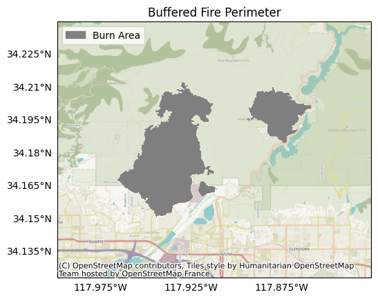
Plotting the perimeter raster, we find it consists of two main burn areas (the Fish and Reservoir fires), with a 3 kilometer buffer along the edges.

# Note: This function may take a bit to download the area basemap
plot.mask(perimeter, title='Buffered Fire Perimeter', legend='Burn Area')

We’ll also save this buffered perimeter for use in later tutorials:

path = perimeter.save('data/buffered-perimeter.tif', overwrite=True)
print_path(path)

.../data/buffered-perimeter.tif

DEM

Next we’ll download a digital elevation model (DEM) dataset for the buffered perimeter. The DEM is often used to (1) design a stream segment network and (2) assess topography characteristics for hazard models. Here, we’ll use the USGS’s 1/3 arc-second DEM, which has a nominal 10 meter resolution.

We can acquire DEM data using the data.usgs.tnm.dem module. Breaking down this namespace:

• usgs collects products distributed by the USGS,

• tnm collects products from The National Map, and

• dem is the module for DEMs from TNM

from pfdf.data.usgs import tnm

DEMs are raster datasets, so we’ll use the read command to load the DEM as a Raster object. We’ll also pass the buffered fire perimeter as the bounds input. This will cause the command to only return data from within the buffered perimeter’s bounding box:

dem = tnm.dem.read(perimeter)

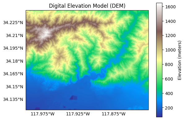
Plotting the DEM, we observe the topography for the assessment area with the San Gabriel mountains to the north, and part of greater Los Angeles in the plain to the south.

plot.raster(dem, cmap='terrain', title='Digital Elevation Model (DEM)', clabel='Elevation (meters)')

We’ll also save the DEM for use in later tutorials:

path = dem.save('data/dem.tif', overwrite=True)
print_path(path)

.../data/dem.tif

STATSGO

Next, we’ll use the data.usgs.statsgo module to download soil characteristic data from the STATSGO archive within the buffered perimeter.

from pfdf.data.usgs import statsgo

Specifically, we’ll download soil KF-factors (KFFACT), which we’ll use to run the M1 likelihood model in the Hazard Assessment Tutorial. We’ll use the read command to load the dataset as a Raster object. Once again, we’ll pass the buffered fire perimeter as the bounds input to only load data within the buffered perimeter’s bounding box:

kf = statsgo.read('KFFACT', bounds=perimeter)

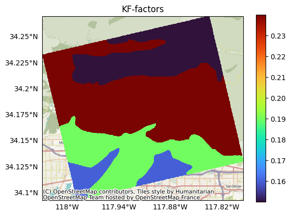
Plotting the KF-factors, we find it consists of values from 0.15 to 0.25 distributed over 4 distinct map units within our assessment domain:

plot.raster(kf, cmap='turbo', title='KF-factors', show_basemap=True)

We’ll also save the KF-factors for use in later tutorials:

path = kf.save('data/kf.tif', overwrite=True)
print_path(path)

.../data/kf.tif

EVT

Next, we’ll download an existing vegetation type (EVT) raster from LANDFIRE. EVTs are often used to locate water bodies, human development, and excluded areas prior to an assessment. Here, we’ll use data from LANDFIRE EVT version 2.4.0, which has a nominal 30 meter resolution.

We can acquire LANDFIRE data using the data.landfire module. Here, we’ll use the read command to read EVT data into memory as a Raster object. The read command requires the name of a LANDFIRE data layer as input. The name of the EVT 2.4.0 layer is 240EVT, and you can find a complete list of LANDFIRE layer names here: LANDFIRE Layers. We’ll also pass the buffered fire perimeter as the bounds input so that the command will only read data from within our assessment domain:

evt = data.landfire.read('240EVT', bounds=perimeter)

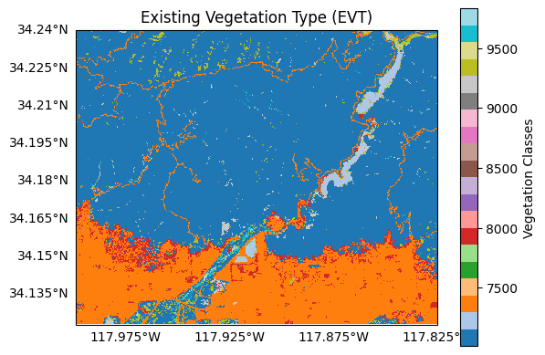
Plotting the dataset, we can observe a variety of classifications. These include:

• A large developed area at the bottom of the map (orange),

• Mostly undeveloped areas throughout the San Gabriel mountains (dark blue),

• Roadways crossing the San Gabriel mountains (orange), and

• Water bodies including the Morris and San Gabriel reservoirs (grey blue).

plot.raster(evt, cmap='tab20', title='Existing Vegetation Type (EVT)', clabel='Vegetation Classes')

We’ll also save the EVT for use in later tutorials:

path = evt.save('data/evt.tif', overwrite=True)
print_path(path)

.../data/evt.tif

Retainment Features

Next, we’ll download the locations of any debris retainment features in our assessment domain. Retainment features are typically human-constructed features designed to catch and hold excess debris. Not all assessment areas will include such features. But when they do, retainment features can be useful for designing the stream segment network, as debris-flows are unlikely to proceed beyond these points.

We can acquire retainment feature locations using data.retainments. Our assessment is in Los Angeles County, so we’ll specifically use the la_county module to do so. Here, we’ll use the download command to download the retainment dataset Geodatabase. By default, the command will download the geodatabase to the current folder, so we’ll use the parent option to save the dataset in our data folder instead. Regardless of where we save the file, the command will always return the absolute path to the downloaded geodatabase as output:

path = data.retainments.la_county.download(parent='data')
print_path(path)

.../data/la-county-retainments.gdb

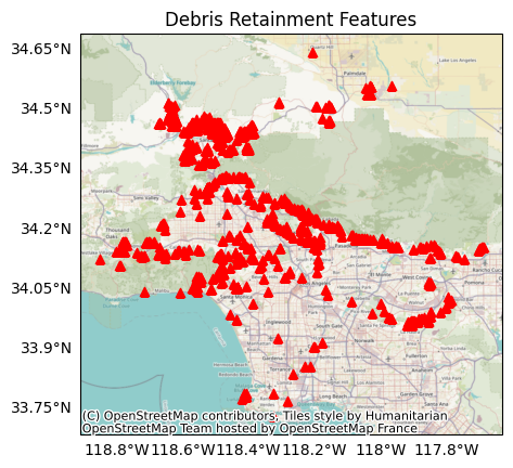
Plotting the retainment features, we observe over 100 retainment points throughout the county:

# Note: May take a bit to download the county basemap
plot.retainments(path, title='Debris Retainment Features')

NOAA Atlas 14

Next, we’ll download rainfall data from NOAA Atlas 14 at the center of our assessment domain. This data is often used to select design storms for running debris-flow hazard assessment models. We can acquire NOAA Atlas 14 data using data.noaa.atlas14. This module requires a latitude and a longitude at which to query rainfall data, so we’ll first reproject the fire perimeter’s bounding box to EPSG:4326 (often referred to as WGS84), and then extract the center coordinate:

bounds = perimeter.bounds.reproject(4326)
lon, lat = bounds.center
print(f'{lon=}, {lat=}')

lon=-117.91205680284118, lat=34.18146282621564

We’ll now use the download command to download rainfall data at this coordinate as a csv file in the current folder. By default, the command will download the dataset to the current folder. We’ll use the parent option to download the file to our data folder instead. Regardless of where we save the file, the command returns the absolute path to the downloaded file as output:

path = data.noaa.atlas14.download(lon=lon, lat=lat, parent='data')
print_path(path)

.../data/noaa-atlas14-mean-pds-intensity-metric.csv

Inspecting the file name, we find this dataset holds mean rainfall intensities in metric units, as calculated using partial duration series (pds). The command also includes options to download min/max values, rainfall depths, values derived from annual mean series (ams), and values in english units. You can learn about these options in the API.

Opening the downloaded file, we find the following data table:

PRECIPITATION FREQUENCY ESTIMATES
ARI (years):,  1, 2, 5, 10, 25, 50, 100, 200, 500, 1000
      5-min:, 61,75,96,114,143,167,195,227,276,319
     10-min:, 44,54,69,82,102,120,140,163,198,229
     15-min:, 35,43,55,66,82,97,113,131,159,184
     30-min:, 24,30,38,46,57,67,78,91,111,128
     60-min:, 18,22,28,33,42,49,57,66,80,93
       2-hr:, 13,16,21,25,31,37,43,50,60,69
       3-hr:, 11,14,18,21,27,31,36,42,51,58
       6-hr:,  8,10,13,16,20,23,27,31,37,43
      12-hr:,  6,7,9,11,14,16,18,21,25,29
      24-hr:,  4,5,6,8,10,11,13,15,18,21
      2-day:,  2,3,4,5,7,8,9,10,13,15
      3-day:,  2,2,3,4,5,6,7,8,10,12
      4-day:,  1,2,3,3,4,5,6,7,8,10
      7-day:,  1,1,2,2,3,3,4,5,6,6
     10-day:,  1,1,1,2,2,3,3,4,4,5
     20-day:,  0,1,1,1,1,2,2,2,2,3
     30-day:,  0,0,1,1,1,1,1,2,2,2
     45-day:,  0,0,1,1,1,1,1,1,1,2
     60-day:,  0,0,0,1,1,1,1,1,1,1

The rows of the table are rainfall durations, and the columns are recurrence intervals of different lengths. The data values are the mean precipitation intensities for rainfall durations over the associated recurrence interval. We can use these values to inform hazard assessment models that require design storms, which is discussed in detail in the hazard assessment tutorial.

Extra Credit: Hydrologic Units

As a bonus exercise, we’ll next download a hydrologic unit data bundle for our assessment domain. Hydrologic units (HUs) divide the US into catchment drainages of various sizes. Each HU is identified using a unique integer code (HUC), where longer codes correspond to smaller units. Many assessments don’t require HU data, but HU boundaries can be useful for large-scale analyses, as they form a natural unit for subdividing assessments.

You can download HU data bundles using the data.usgs.tnm.nhd module. Breaking down this namespace:

• usgs collects products distributed by the USGS,

• tnm collects products from The National Map, and

• nhd is the module for the National Hydrologic Dataset, which collects the HUs.

We’ll specifically use the nhd.download command, which requires an HUC4 or HUC8 code as input. Note that you must input HUCs as strings, rather than ints. (This is to support HUCs with leading zeros). Much of the San Gabriel assessment falls in HU 18070106, so we’ll download the data bundle for that HU. By default, the command will download its data bundle to the current folder, so we’ll use the parent option to download the bundle to our data folder instead:

path = data.usgs.tnm.nhd.download(huc='18070106', parent='data')
print_path(path)

.../data/huc8-18070106

From the output file path, we find the data bundle has been downloaded to a folder named “huc8-18070106”. Inspecting the folder’s contents, we find it contains a variety of Shapefile data layers in an internal Shape subfolder.

print_contents(path/"Shape", extension=".shp")

['NHDArea.shp', 'NHDAreaEventFC.shp', 'NHDFlowline.shp', 'NHDLine.shp', 'NHDLineEventFC.shp', 'NHDPoint.shp', 'NHDPointEventFC.shp', 'NHDWaterbody.shp', 'WBDHU10.shp', 'WBDHU12.shp', 'WBDHU14.shp', 'WBDHU16.shp', 'WBDHU2.shp', 'WBDHU4.shp', 'WBDHU6.shp', 'WBDHU8.shp', 'WBDLine.shp']

Although the download command will only accept HU4 and HU8 codes, it’s worth noting that the data bundle includes watershed boundaries for HUs 2 through 16. We will not use these datasets in the tutorials, but we note that HU10 boundaries can often be a good starting point for large-scale analyses.

Conclusion

In this tutorial, we’ve learnen how to use download and read commands in pfdf.data to load various datasets from the internet. These commands can help automate data acquisition for assessments, once initial datasets like the fire perimeter have been acquired. In this tutorial, we’ve downloaded datasets with a variety of resolutions and spatial projections. In the next tutorial, we’ll learn ways to clean and reproject these datasets prior to an assessment.

Quick Reference

This quick reference script collects the commands explored in the tutorial:

# Resets this notebook for the script
workspace.remove_downloads()
%reset -f

Cleaned workspace of downloaded datasets

from pfdf import data
from pfdf.raster import Raster

# Build a buffered burn perimeter
perimeter = Raster.from_polygons('data/perimeter.geojson')
perimeter.buffer(3, 'kilometers')

# Load a DEM into memory
dem = data.usgs.tnm.dem.read(bounds=perimeter)

# Load STATSGO soil data into memory
kf = data.usgs.statsgo.read('KFFACT', bounds=perimeter)

# Load a LANDFIRE EVT into memory
evt = data.landfire.read('240EVT', bounds=perimeter)

# Download retainment features
retainments_path = data.retainments.la_county.download(parent='data')

# Download NOAA Atlas 14 data
bounds = perimeter.bounds.reproject(4326)
lon, lat = bounds.center
atlas14_path = data.noaa.atlas14.download(lon=lon, lat=lat, parent='data')

# Download a hydrologic unit data bundle
huc_path = data.usgs.tnm.nhd.download(huc='18070106', parent='data')