Preprocessing Tutorial

This tutorial demonstrates how to use Raster routines to clean and reproject datasets for an assessment. Or skip to the end for a quick reference script.

Introduction

Many pfdf routines use multiple raster datasets as input. When this is the case, pfdf usually requires the rasters to have the same shape, resolution, CRS, and alignment. Some routines also require data values to fall within a valid data range. However, real datasets are rarely this clean, and so the Raster class provides commands to help achieve these requirements.

In this tutorial, we’ll apply preprocessing routines to the input rasters for a real hazard assessment - the 2016 San Gabriel Fire Complex in California.

Prerequisites

Install pfdf

To run this tutorial, you must have installed pfdf 3+ with tutorial resources in your Jupyter kernel. The following line checks this is the case:

import check_installation

pfdf and tutorial resources are installed

Download Data Tutorial

This tutorial uses datasets that are downloaded in the Download Data Tutorial. If you have not run that tutorial, then you should do so now. The following line checks the required datasets have been downloaded:

from tools import workspace
workspace.check_datasets()

The required datasets are present

Imports

Next, we’ll import the Raster class, which we’ll use to load and preprocess the datasets. We’ll also import pathlib.Path, which we’ll use to manipulate file paths; and the plot module, which we’ll use to visualize the datasets.

from pfdf.raster import Raster
import numpy as np
from pathlib import Path
from tools import plot

Datasets

Inputs

In this tutorial we’ll preprocess the following datasets:

Dataset	Description	Type	EPSG	Resolution	Source
perimeter	Fire burn perimeter	MultiPolygon	26911	NA	User provided
dem	Digital elevation model (10 meter resolution)	Raster	4269	10 meter	data.usgs.tnm.dem
dnbr	Differenced normalized burn ratio	Raster	26911	10 meter	User provided
kf	Soil KF-factors	Raster	5069	30 meter	data.usgs.statsgo
evt	Existing vegetation type	Raster	5070	30 meter	data.landfire
retainments	Debris retainment features	MultiPoint	4326	NA	data.retainments.la_county

As can be seen from the table, these datasets are in a variety of formats (Raster, Polygons, Points), use 5 different CRS, and have several different resolutions. The aim of this tutorial is to convert these datasets to rasters with the same CRS, resolution, and bounding box. Specifically, the preprocessed rasters will have the following characteristics:

Characteristic	Value	Note
EPSG	4269	Matches the DEM
Resolution	10 meter	Hazard models were calibrated using 10 meter DEMs
Bounding Box		Will match the buffered fire perimeter

We’ll also ensure that certain datasets (dnbr and kf) fall within valid data ranges.

Derived

We’ll also produce the following new datasets from the inputs:

Derived Dataset	Description	Source
severity	Soil burn severity	Estimated from dNBR
iswater	Water body mask	Derived from EVT
isdeveloped	Human development mask	Derived from EVT

These datasets are typically considered inputs to the hazard assessment process, hence their inclusion in the preprocessing stage.

Important!

Hazard assessments should use field validated soil burn severity whenever possible. We use a derived value here to demonstrate how this dataset can be estimated when field-validated data is not available.

Acquire Data

In many hazard assessments, you’ll need to provide the fire perimeter and dNBR raster. You’ll also often provide the soil burn severity, but we’ve deliberately neglected that dataset in this tutorial.

As we saw in the data tutorial, the analysis domain is typically defined by a buffered fire perimeter. The perimeter is buffered so that the assessment will include areas downstream of the burn area. Let’s start by loading the buffered burn perimeter and dNBR:

perimeter = Raster.from_file('data/buffered-perimeter.tif')
dnbr = Raster.from_file('data/dnbr.tif')

In the data tutorial, we also saw how you can use pfdf.data to download several commonly-used raster datasets. These included USGS DEMs, STATSGO soil KF-factors, and LANDFIRE EVTs. We already downloaded these datasets in the data tutorial, so let’s load them now:

dem = Raster.from_file('data/dem.tif')
evt = Raster.from_file('data/evt.tif')
kf = Raster.from_file('data/kf.tif')

We also used pfdf.data to download several non-raster datasets. Of these, we’re particularly interested in the debris retainment features, as hazard assessments can use these to design the stream segment network. The downloaded debris retainment features are a Point feature collection - this is not a raster dataset, so we’ll just get the path to the dataset for now:

retainments_path = 'data/la-county-retainments.gdb'

Rasterize Debris Retainments

Hazard assessments require most datasets to be rasters, so we’ll need to rasterize any vector feature datasets before proceeding. The debris retainments are vector features - specifically, a collection of Point geometries - so we’ll rasterize them here.

You can convert Point or MultiPoint features to a Raster object using the from_points factory. We’ll only introduce the factory here, but you can find a detailed discussion in the Raster Factories Tutorial. In brief, this command takes the path to a Point feature file, and converts the dataset to a raster. By default, the rasterized dataset will have a resolution of 10 meters, which is the recommended resolution for standard hazard assessments.

Before calling the from_points command, let’s compare the retainment dataset to the fire perimeter. Here, red triangles are retainment features, and the fire perimeter is the dark grey area right of center:

plot.retainments(
    retainments_path, 
    perimeter=perimeter, 
    title='Retainments + Fire Perimeter'
)

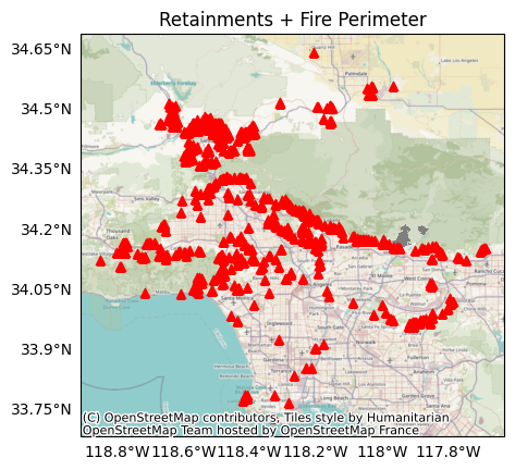
Examining the plot, we find the Point dataset covers a much larger area than the fire perimeter. Converting the full retainment dataset to a raster would require a lot of unnecessary memory, so we’ll use the bounds option to only rasterize the dataset within the buffered fire perimeter:

retainments = Raster.from_points(retainments_path, bounds=perimeter)

Reprojection

Our next task is to project the rasters into the same CRS. As we saw in the table above, they currently use 5 different CRSs. We’ll select the CRS of the DEM dataset as our target CRS. This is because high-fidelity DEM data is essential for determining flow pathways, and using the DEM CRS will keep this dataset in its original state.

You can reproject a Raster object using its built-in reproject method. In addition to matching CRSs, we also want our datasets to have the same alignment and resolution, and the reproject command can do this as well. Here, we’ll use the template option to reproject each dataset to match the CRS, resolution, and alignment

rasters = [perimeter, dem, dnbr, kf, evt, retainments]
for raster in rasters:
    raster.reproject(template=dem)

Inspecting the rasters, we find they now all have the same CRS:

for raster in rasters:
    print(raster.crs.name)

NAD83
NAD83
NAD83
NAD83
NAD83
NAD83

This tutorial only uses the template option for the reproject command, but there are also other options, such as the choice of resampling algorithm. As a reminder, you can learn about commands in greater detail in the User Guide and API.

Clipping

Our next task is to clip the rasters to the same bounding box. The current bounding boxes are similar, but can differ slightly due to the reprojection. You can clip a Raster object to a specific bounding box using its built-in clip method. Here, we’ll use the buffered fire perimeter as the target bounding box, since the perimeter defines the domain of the hazard assessment:

for raster in rasters:
    raster.clip(bounds=perimeter)

Inspecting the rasters, we find they now all have the same bounding box:

for raster in rasters:
    print(raster.bounds)

BoundingBox(left=-117.99879629663243, bottom=34.123055554762374, right=-117.82527777792725, top=34.23981481425213, crs="NAD83")
BoundingBox(left=-117.99879629663243, bottom=34.123055554762374, right=-117.82527777792725, top=34.23981481425213, crs="NAD83")
BoundingBox(left=-117.99879629663243, bottom=34.123055554762374, right=-117.82527777792725, top=34.23981481425213, crs="NAD83")
BoundingBox(left=-117.99879629663243, bottom=34.123055554762374, right=-117.82527777792725, top=34.23981481425213, crs="NAD83")
BoundingBox(left=-117.99879629663243, bottom=34.123055554762374, right=-117.82527777792725, top=34.23981481425213, crs="NAD83")
BoundingBox(left=-117.99879629663243, bottom=34.123055554762374, right=-117.82527777792725, top=34.23981481425213, crs="NAD83")

Data Ranges

It’s often useful to constrain a dataset to a valid data range, and you can use a Raster object’s set_range command to do so. We’ll do this for the dNBR and KF-factor datasets.

dNBR

There is no “correct” range for dNBR values, but -1000 to 1000 is a reasonable interval. Inspecting our dNBR data, we find it includes some values outside of this interval:

data = dnbr.values[dnbr.data_mask]
print(min(data))
print(max(data))

-1350
1500

Here, we’ll use the set_range command to constrain the dNBR raster to our desired interval. In this base syntax, data values outside this range will be set to the value of the nearest bound. (NoData pixels are not affected):

dnbr.set_range(min=-1000, max=1000)

Inspecting the dataset again, we find that the data values are now within our desired interval:

data = dnbr.values[dnbr.data_mask]
print(min(data))
print(max(data))

-1000
1000

KF-factors

We’ll also constrain the KF-factor raster to positive values, as negative KF-factors are unphysical. The STATSGO dataset sometimes uses -1 values to mark large water bodies with missing data, but -1 is not the NoData value, so these -1 values appear as unphysical data values that should be removed from the dataset.

We’ll use the set_range command to ensure the dataset does not include any such values. Here, we’ll use the fill option, which will replace out-of-bounds data values with NoData, rather than setting them to the nearest bound. We’ll also use the exclude_bounds option, which indicates that the bound at 0 is not included in the valid data range, so should also be converted to NoData:

kf.set_range(min=0, fill=True, exclude_bounds=True)

Inspecting the raster, we find it does not contain unphysical data values:

data = kf.values[kf.data_mask]
print(min(data))

0.15

Estimate Severity

Many hazard assessments will require a BARC4-like soil burn severity (SBS) dataset. In brief, a BARC4 dataset classifies burned areas as follows:

Value	Description
1	Unburned
2	Low burn severity
3	Moderate burn severity
4	High burn severity

This dataset should be sourced from field-validated data when possible, but sometimes such datasets are not available. For example, SBS is often not available for preliminary assessments conducted before a fire is completely contained. When this is the case, you can estimate a BARC4-like SBS from a dNBR or other dataset using the severity.estimate command. Let’s do that here. We’ll start by importing pfdf’s severity module:

from pfdf import severity

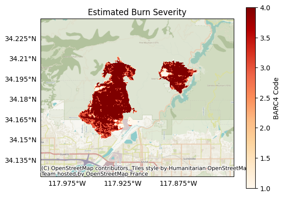
Next we’ll use the estimate command to estimate a BARC4 from the dNBR. This command allows you to specify the thresholds between unburned and low, low and moderate, and moderate and high severity. Here, we’ll use thresholds of 125, 250, and 500 to classify the dNBR dataset into BARC4 values:

barc4 = severity.estimate(dnbr, thresholds=[125,250,500])

Plotting the new dataset, we observe it has classified the dNBR into 4 groups, as per our thresholds:

plot.raster(
    barc4, 
    cmap='OrRd', 
    title='Estimated Burn Severity', 
    clabel='BARC4 Code', 
    show_basemap=True
)

Terrain Masks

Our final task is to build terrain masks from the EVT dataset. Specifically, we want to locate water bodies and human development. Debris flows are unlikely to initiate in water bodies, so it will be useful to exclude them from the hazard assessment. Similarly, human development can alter debris-flow behavior in ways outside the scope of the assessment models, so we’ll locate these areas from the assessment as well. The EVT dataset uses different integer codes to classify terrain. The code for water bodies is 7292, and human development is marked by the integers from 7296 to 7300.

You can locate specific values in a Raster object using the find method. This method returns a boolean raster mask that locates the queried values in the initial raster. True values indicate pixels that match one of the queried values, and all other pixels are marked as False. Let’s use the find command to build our water and development masks:

iswater = evt.find(7292)
isdeveloped = evt.find([7296, 7297, 7298, 7299, 7300])

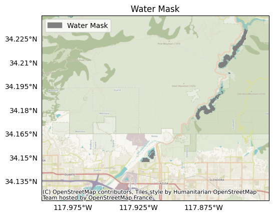
Plotting the water mask, we find it marks pixels in the Morris and San Gabriel reservoirs:

plot.mask(iswater, title='Water Mask', legend='Water Mask')

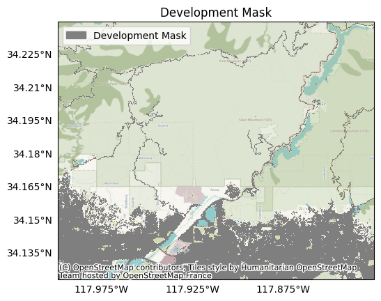
And the development mask marks roadways and greater Los Angeles:

plot.mask(isdeveloped, title='Development Mask')

Save Preprocessed Datasets

We’ll now save our preprocessed rasters so we can use them in later tutorials. We’ll start by creating a folder for the preprocessed datasets to disambiguate them from the raw datasets in the data folder:

folder = Path.cwd() / 'preprocessed'
folder.mkdir(exist_ok=True)

Then, we’ll collect and save the preprocessed rasters:

rasters = {
    'perimeter': perimeter,
    'dem': dem,
    'dnbr': dnbr,
    'barc4': barc4,
    'kf': kf,
    'retainments': retainments,
    'evt': evt,
    'iswater': iswater,
    'isdeveloped': isdeveloped,
}
for name, raster in rasters.items():
    raster.save(f'preprocessed/{name}.tif', overwrite=True)

Conclusion

In this tutorial, we’ve learned how to preprocess datasets for an assessment. We

• Rasterized vector datasets,

• Reprojected to the same CRS,

• Clipped to the same bounding box,

• Constrained data ranges,

• Estimated severity, and

• Located terrain masks.

In the next tutorial, we’ll learn how to leverage these datasets to implement a hazard assessment.

Quick Reference

This quick reference script collects the commands explored in the tutorial:

# Resets this notebook for the script
%reset -f

from pathlib import Path
import numpy as np
from pfdf.raster import Raster
from pfdf import severity

# Load datasets
perimeter = Raster.from_file('data/buffered-perimeter.tif')
dem = Raster.from_file('data/dem.tif')
dnbr = Raster.from_file('data/dnbr.tif')
kf = Raster.from_file('data/kf.tif')
evt = Raster.from_file('data/evt.tif')

# Rasterize debris retainments
retainments = Raster.from_points('data/la-county-retainments.gdb', bounds=perimeter)

# Reproject rasters to match the DEM projection
rasters = [perimeter, dem, dnbr, kf, evt, retainments]
for raster in rasters:
    raster.reproject(template=dem)

# Clip rasters to the bounds of the buffered perimeter
for raster in rasters:
    raster.clip(bounds=perimeter)

# Constrain data ranges
dnbr.set_range(min=-1000, max=1000)
kf.set_range(min=0, fill=True, exclude_bounds=True)

# Estimate severity
barc4 = severity.estimate(dnbr, thresholds=[125,250,500])

# Build terrain masks
iswater = evt.find(7292)
isdeveloped = evt.find([7296, 7297, 7298, 7299, 7300])