Hazard Assessment Tutorial

This tutorial shows how to use pfdf to implement a hazard assessment. Or skip to the end for a quick reference script.

Introduction

Now that we’ve acquired and preprocessed our datasets, we’re finally ready to implement a hazard assessment. In this tutorial we’ll follow a typical USGS hazard assessment. In brief, the assessment will include the following steps:

• Characterize the watershed,

• Design a stream segment network,

• Run hazard models on stream segments, and

• Export results to common GIS formats.

Stream Segment Network

A stream segment network is a collection of flow pathways across a landscape, and these flow paths approximate the local drainage networks. When two stream segments meet, the two segments end and a new segment begins at the confluence point. Stream segments form the basis of USGS-style hazard assessments. In these assessments, hazard models are run on each segment, using information derived from the segment’s flow path and catchment basin.

In the tutorial, we’ll start by delineating an initial stream segment network. We’ll design this network to exclude areas that aren’t at elevated risk of debris-flow hazards. For example, the initial network will exclude segments that aren’t downstream of the burn area.

After delineating the initial network, we’ll next refine the network, filtering it to a final collection of model-worthy stream segments. These final segments will be selected to meet various physical criteria for elevated debris-flow risk. For example, the final network will not contain stream segments with very large catchment areas, as large catchments tend to exhibit flood-like flows, rather than debris flow-like behavior.

Hazard Models

We will use a total of 4 hazard models in this tutorial. These include:

• Potential sediment volume,

• Debris-flow likelihood,

• Combined hazard classification, and

• Rainfall thresholds.

We’ll then estimate potential sediment volumes using the Gartner et al., 2014 emergency model. This model uses terrain and fire severity data to estimate potential sediment volume given a set of design peak 15-minute rainfall intensities. These rainfall intensities are sometimes referred to as design storms, and should be selected to reflect potential future rainfall scenarios in the burn area. We also note that pfdf also supports the Gartner 2014 longterm assessment model, but we will not discuss this in the tutorial.

Next, we’ll estimate debris-flow likelihoods using the M1 model of Staley et al., 2017. This model uses terrain, fire severity, and soil data to estimate debris-flow likelihoods given a set of design rainfall intensities. Here, we’ll use the same design storms used for the volume model. The pfdf library also supports the M2, M3, and M4 models, but we will not discuss them in the tutorial.

We’ll then use a combined hazard classification to estimate the relative hazard of each stream segment and catchment basin. Here, we’ll use a modification of the classification scheme presented by Cannon et al., 2010. This scheme considers both debris-flow likelihood and volume to estimate relative hazard.

Finally, we’ll apply a rainfall threshold model to determine rainfall levels that are likely to cause debris flow events. Unlike the previous levels, this model estimates rainfall levels as output, rather than using design storms as an input parameter. We’ll specifically use the inverted M1 model, which estimates the rainfall levels needed to achieve design probability levels for debris-flow events.

Prerequisites

Install pfdf

To run this tutorial, you must have installed pfdf 3+ with tutorial resources in your Jupyter kernel. The following line checks this is the case:

import check_installation

pfdf and tutorial resources are installed

Preprocessing Tutorial

This tutorial uses datasets prepared in the Preprocessing Tutorial. If you have not run that tutorial, then you should do so now. The following line checks the required datasets have been downloaded:

from tools import workspace
workspace.check_preprocessed()

The preprocessed datasets are present

Imports

We’ll need to import many different pfdf components to implement the hazard assessment. We’ll defer these imports to the associated sections below to help with organization. For now, we’ll just import a few tools used to run the tutorial:

from tools import plot, print_path

Load Preprocessed Data

Our first step is to load the preprocessed datasets. We’ll do this with the Raster class, using the from_file factory. We’ll use the isbool option for several datasets so they are correctly loaded as boolean masks, rather than as integers:

from pfdf.raster import Raster

perimeter = Raster.from_file('preprocessed/perimeter.tif', isbool=True).values
dem = Raster.from_file('preprocessed/dem.tif')
dnbr = Raster.from_file('preprocessed/dnbr.tif')
kf = Raster.from_file('preprocessed/kf.tif')
barc4 = Raster.from_file('preprocessed/barc4.tif')
iswater = Raster.from_file('preprocessed/iswater.tif', isbool=True).values
isdeveloped = Raster.from_file('preprocessed/isdeveloped.tif', isbool=True)
isretainment = Raster.from_file('preprocessed/retainments.tif', isbool=True)

Characterize Watershed

Next, we’ll characterize the watershed in our area of interest. Specifically, we will locate areas burned at various severities, determine flow directions, and compute various physical properties. This characterization will help us (1) delineate the stream segment network, and (2) quantify terrain and fire severity variables for hazard models.

Burn Severity Masks

We’ll begin the watershed characterization by building two burn severity masks. The first mask will locate all pixels that were burned at any level. The second mask will locate pixels that were burned at moderate-or-high severity.

You can build severity masks using the mask function in the severity module:

from pfdf import severity

This function takes a BARC4-like raster as input and returns a raster mask for the queried burn severity levels:

isburned = severity.mask(barc4, "burned")
moderate_high = severity.mask(barc4, ["moderate", "high"])

Flow Directions

Next, we’ll use the watershed module to analyze the watershed.

from pfdf import watershed

We’ll start by using a conditioned DEM to compute flow directions.

conditioned = watershed.condition(dem)
flow = watershed.flow(conditioned)

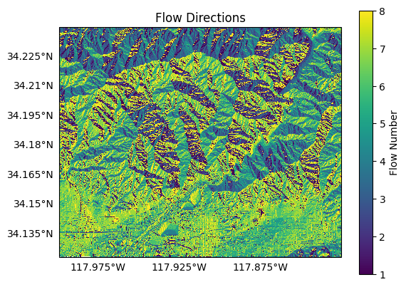
The output flow direction raster uses the integers from 1 to 8 to mark flow directions. For pixel X, flow is denoted as follows:

\[\begin{split} \begin{matrix} 4 & 3 & 2\\ 5 & \mathrm{X} & 1\\ 6 & 7 & 8\\ \end{matrix} \end{split}\]

For example, if pixel X flow to the pixel up and left, then the flow number for pixel X will be 3. Plotting our flow direction raster, we can get a rough sense of the flow planes in our watershed:

plot.raster(flow, cmap='viridis', title='Flow Directions', clabel='Flow Number')

We’ll then use the flow directions to compute physical properties for the watershed. Specifically, we’ll determine each pixel’s flow slope, and its vertical relief to the nearest ridge cell:

slopes = watershed.slopes(conditioned, flow)
relief = watershed.relief(conditioned, flow)

Flow Accumulation

Finally, we’ll use the watershed.accumulation function to compute several types of flow accumulations. By default, the accumulation function will count the number of upstream pixels for each point on the raster. However, you can use the mask option to only count upstream pixels that meet the mask criterion instead. For example, we’ll start by using the retainment feature mask to count the number of retainments above each pixel:

nretainments = watershed.accumulation(flow, mask=isretainment)

We’ll then compute the total catchment area, and total burned catchment area for each pixel. Here, we’ll use the times option to multiply pixel counts by the area of a raster pixel. This way, the area rasters will both have units of square kilometers, rather than pixel counts:

pixel_area = dem.pixel_area(units='kilometers')
area = watershed.accumulation(flow, times=pixel_area)
burned_area = watershed.accumulation(flow, mask=isburned, times=pixel_area)

Stream Segment Network

We’ll next design a stream segment network using the Segments class from the pfdf.segments package:

from pfdf.segments import Segments

Delineation Mask

To create a stream segment network, we’ll first require a network delineation mask. This mask is used to exclude non-viable pixels from the network. False pixels will never be included in a stream segment. By contrast, a True pixel may be included in the network, but there’s no guarantee.

As a starting point, most masks should exclude pixels with catchments that are too small to generate a debris flow. We’ll also exclude catchments that are negligibly burned, as these areas are unlikely to exhibit altered debris-flow hazards. Finally, we’ll exclude pixels below debris-flow retainment features, as debris flows are unlikely to proceed beyond these points.

We’ll start by defining two parameters:

min_area_km2 = 0.025
min_burned_area_km2 = 0.01

Here, min_area_km2 defines the minimum catchment area (in square kilometers). Smaller catchments are usually too small to be able to generate a debris-flow. The min_burned_area_km2 parameter defines the minimum burned catchment area (also square kilometers). Catchments with smaller burned areas are negligibly affected by the fire. We can compare these thresholds to the flow accumulation rasters to help build several criteria masks:

large_enough = area.values >= min_area_km2
below_burn = burned_area.values >= min_burned_area_km2
below_retainment = nretainments.values > 0

Here, large_enough indicates catchments that are large enough to generate debris flows, and below_burn indicates catchments that are sufficiently burned as to have elevated debris-flow risk. Finally, below_retainment indicates areas that are below a retainment feature, and therefore are shielded from debris flows.

We can use these criteria to build the final delineation mask. First we’ll define “at risk” areas as anywhere within or downstream of the burn area:

at_risk = perimeter | below_burn

Then, we’ll set the delineation mask to include catchments that are sufficiently large and “at risk”, but to exclude water bodies and catchments shielded by retainment features:

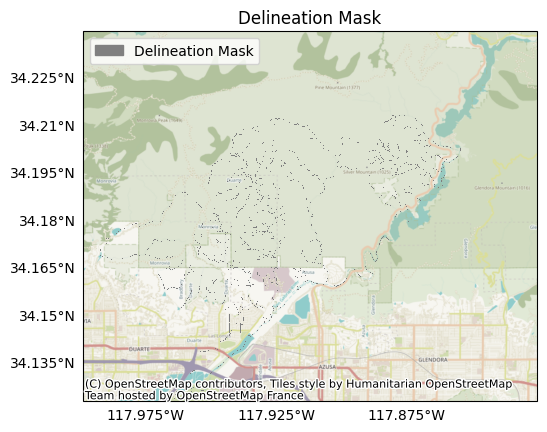
mask = large_enough & at_risk & ~iswater & ~below_retainment

Plotting the delineation mask, we find it consists of various stream pathways in and around the burn area. Because this figure has a lower resolution than the actual mask, the plot may look like a series of disjointed pixels. But in reality, most of the pixels connect continuously:

plot.mask(mask, title='Delineation Mask', spatial=dem)

Delineate Network

We’re just about ready to delineate the stream network. Let’s define one additional parameter first:

max_length_m = 500

This parameter establishes a maximum length for segments in the network (in meters). Segments longer than this length will be split into multiple pieces. We can now use the Segments constructor to delineate the network. This will return a new Segments object that manages our network:

segments = Segments(flow, mask, max_length_m)

Inspecting the object, we find the stream network consists of 696 stream segments, which are distributed in 41 local drainage networks.

print(segments)

Segments:
    Total Segments: 696
    Local Networks: 41
    Located Basins: False
    Raster Metadata:
        Shape: (1261, 1874)
        CRS("NAD83")
        Transform(dx=9.259259269219641e-05, dy=-9.25925927753796e-05, left=-117.99879629663243, top=34.23981481425213, crs="NAD83")
        BoundingBox(left=-117.99879629663243, bottom=34.123055554762374, right=-117.82527777792725, top=34.23981481425213, crs="NAD83")

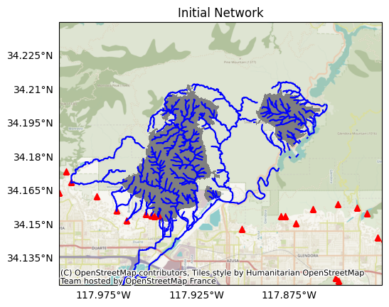
Plotting the network, we finde the segments are distributed in and around the fire perimeter. Here, blue lines are stream segments, the fire perimeter is in grey, and red triangles indicate retainment features:

plot.network(segments, title='Initial Network', perimeter=perimeter, show_retainments=True)

Filter Network

Next, we’ll refine the network to a collection of model-worthy segments. We’ll do this by filtering out segments that don’t meet various physical criteria for debris-flow risk. Here, we’ll consider:

---

Catchment Area

Segments with very large catchments will likely exhibit flood-like behavior, rather than debris-flow like. As such, we’ll remove segments with very large catchments.

Burn Ratio

The catchment must be sufficiently burned, or it will be negligibly affected by the fire. Here, we’ll remove segments whose catchments are insufficiently burned.

Slope

Debris flows are most common in areas with steep slopes, as shallow slopes can lead to sediment deposition, rather than debris flow. We’ll remove segments whose slopes are too shallow.

Confinement Angle

Debris flows are more common in confined areas, as open areas can allow debris deposition, rather than flow. We’ll remove segments that are insufficiently confined.

Developed Area

Human development can alter the course and behavior of debris flows, so we’ll remove segments that contain large amounts of human development.

---

With the exception of catchment area, we will only filter segments that are outside of the fire perimeter. Segments within the perimeter will be retained, regardless of physical characteristics. We make this choice because removing segments in the perimeter can result in assessment maps that appear incomplete to stakeholders unfamiliar with the assessment process. Ultimately, retaining all segments in the perimeter tends to reduce stakeholder confusion.

We’ll start by defining several filtering parameters:

min_burn_ratio = 0.25
min_slope = 0.12
max_area_km2 = 8
max_developed_area_km2 = 0.025
max_confinement = 174
neighborhood = 4

Most of these parameters define a threshold for one of the filtering checks. The final neighborhood parameter indicates the pixel radius of the focal window used to compute confinement angles.

Next, we’ll use the segments object to compute the filtering variables for each segment. Note that the area and developed_area commands return values in square kilometers by default:

area_km2 = segments.area(units='kilometers')
burn_ratio = segments.burn_ratio(isburned)
slope = segments.slope(slopes)
confinement = segments.confinement(dem, neighborhood)
developed_area_km2 = segments.developed_area(isdeveloped)
in_perimeter = segments.in_perimeter(perimeter)

Here, the output variables are 1D numpy arrays with one element per segment in the network. For example, inspecting the area_km2 array gives us the total catchment area for each segment. (Note that we’re only showing values for the first 10 segments here):

print(area_km2[:10])

[0.30236611 0.31429238 2.45540925 0.21195443 0.10286411 0.61665849
 0.91507841 3.9632936  4.2709213  4.4911189 ]

We’ll then compare the variables to the thresholds. The resulting arrays are boolean vectors with one element per segment:

floodlike = area_km2 > max_area_km2
burned = burn_ratio >= min_burn_ratio
steep = slope >= min_slope
confined = confinement <= max_confinement
undeveloped = developed_area_km2 <= max_developed_area_km2

For example, we can inspect the burned array to determine which segments have sufficiently burned catchments. Here, we find that segment 5 has a sufficiently burned catchment:

print(burned[:10])

[False False False False  True False False False False False]

Finally, we’ll use these arrays to filter the network. We’ll remove all flood-like segments, and we’ll retain any segments that :

• Are in the fire perimeter,

• Meet physical criteria for debris-flow risk, or

• Would cause a flow discontinuity if removed.

We use the continuous function to implement the final criteria. In its default configuration, it will return a boolean vector indicating the segments that either (A) were indicated should be kept, or (B) should be kept to preserve flow continuity.

at_risk = burned & steep & confined & undeveloped
keep = ~floodlike & (in_perimeter | at_risk)
keep = segments.continuous(keep)

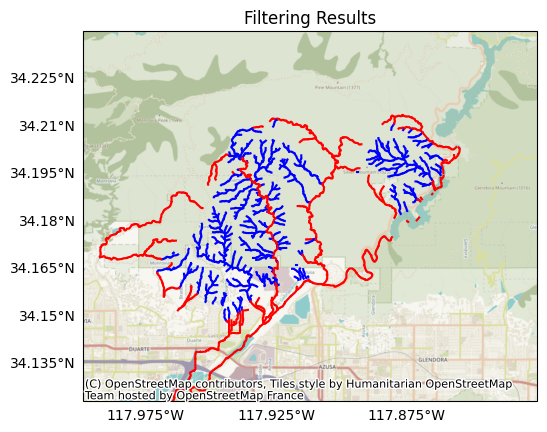
Let’s visualize the filtering results - segments being retained are in blue, and segments being removed are in red. For the most part, the segments being removed either have very large catchments (and anticipated flood-like behavior), or they are on relatively flat terrain:

plot.network(segments, title='Filtering Results', keep=keep)

We’ll filter the network to our preferred segments using the keep command. Inspecting the network afterward, we find the network has been reduced to 460 segments in 92 local drainage networks:

segments.keep(keep)
print(segments)

Segments:
    Total Segments: 460
    Local Networks: 92
    Located Basins: False
    Raster Metadata:
        Shape: (1261, 1874)
        CRS("NAD83")
        Transform(dx=9.259259269219641e-05, dy=-9.25925927753796e-05, left=-117.99879629663243, top=34.23981481425213, crs="NAD83")
        BoundingBox(left=-117.99879629663243, bottom=34.123055554762374, right=-117.82527777792725, top=34.23981481425213, crs="NAD83")

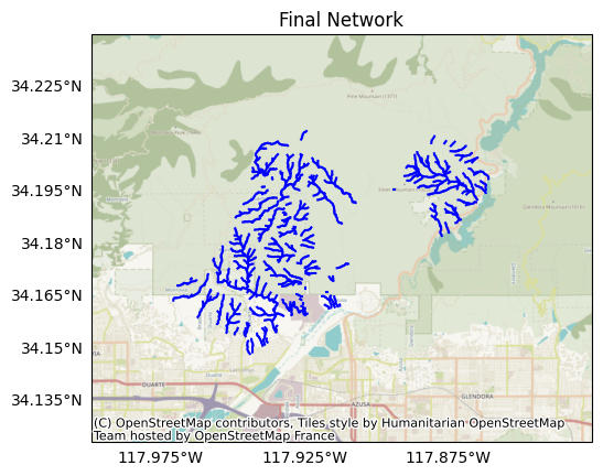
Plotting the network, we find it now only includes of our preferred stream segments:

plot.network(segments, title='Final Network')

Hazard Models

We’ve finished designing the stream network, so we’re now ready to implement the hazard models.

Volume

We’ll start with the potential sediment volume model. As a reminder, we’ll be using the emergency assessment model from Gartner et al., 2014. You can implement the models from this paper using the models.g14 module:

from pfdf.models import g14

The emergency assessment volume model uses terrain and fire severity data to estimate sediment volume. The model also requires a set of selected peak 15-minute rainfall intensities (mm/hour), often referred to as “design storms”. We’ll start by selecting some design rainfall intensities for our assessment. Looking back at the NOAA Atlas 14 data we downloaded in the data tutorial, we find that - within our area of interest - the peak 15-minute rainfall intensity for a 1 year recurrence interval is 35 mm/hour. We’ll run the model for 35 mm/hour and also several adjacent values to capture a range of potential storm scenarios:

I15_mm_hr = [16, 24, 35, 40]

These values are reasonable for the San Gabriel assessment area, but other assessments will likely need different design storm values. As we saw in the Data Tutorial, you can use the data.noaa.atlas14 to download rainfall recurrence intervals for an area, and there are many other useful rainfall datasets online.

The volume model also requires terrain and fire severity data for each stream segment. Specifically, it requires each segment’s vertical relief (relief), and the total catchment area burned at moderate-or-high intensity (Bmh_km2). We can use the segments object to compute these variables given various watershed characteristics:

Bmh_km2 = segments.burned_area(moderate_high)
relief = segments.relief(relief)

Here, each variable is a 1D numpy array with one value per segment in the network. We can now use the g14.emergency function to run the volume model:

volumes, Vmin, Vmax = g14.emergency(I15_mm_hr, Bmh_km2, relief)

Here, volumes holds the central volume estimates, and Vmin and Vmax are the upper and lower bounds of the 95% confidence interval. The outputs are 2D arrays: each row is a stream segment, and each column holds the results for a design storm.

print(volumes.shape)
print((segments.size, len(I15_mm_hr)))

(460, 4)
(460, 4)

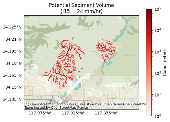
Let’s visualize the results for a design storm with a peak 15-minute rainfall intensity of 24 mm/hour (V[:,1]):

k = 1 # The index of the design storm we are plotting
plot.volumes(segments, volumes[:,k], title='Potential Sediment Volume', I15=I15_mm_hr[k], clabel='Cubic meters')

Likelihood

Next, we’ll use the M1 model from Staley et al., 2017 to estimate debris-flow likelihoods. You can implement the models from this paper using the models.s17 module:

from pfdf.models import s17

As a reminder, this model uses terrain, fire severity, and soil data to estimate debris-flow likelihoods given a set of design storms. The M1 model supports design storms for multiple rainfall durations, but we’ll limit ourselves to the same 15-minute rainfall intensities used to run the volume model. This way, the likelihood and volume results will be comparable, which is required to classify combined hazard:

print(I15_mm_hr)

[16, 24, 35, 40]

The model is calibrated to different parameters for different rainfall durations, so we’ll first query the calibration parameters for 15-minute intervals:

B, Ct, Cf, Cs = s17.M1.parameters(durations=15)

These are the model intercept B, and coefficients for the terrain Ct, fire Cf, and soil Cs variables. Also, the M1 model expects rainfall accumulations, not intensities, so we’ll need to use the intensity module to convert our design storms to accumulations:

from pfdf.utils import intensity
R15 = intensity.to_accumulation(I15_mm_hr, durations=15)

Inspecting these values, we cfind they’ve been divided by 4 to convert from 15-minute intensities to accumulations:

print(R15)

[ 4.    6.    8.75 10.  ]

Next, the model requires terrain, fire severity, and soil data. Specifically, these are:

• Terrain: The proportion of catchment area with both (1) moderate-or-high burn severity, and (2) a slope angle of at least 23 degrees

• Fire: Mean catchment dNBR divided by 1000

• Soil: Mean catchment KF-factor

We can compute these by calling the s17.M1.variables method with various input datasets:

T, F, S = s17.M1.variables(segments, moderate_high, slopes, dnbr, kf, omitnan=True)

Now that we’ve collected our inputs, we can run the model using the s17.likelihood function:

likelihoods = s17.likelihood(R15, B, Ct, T, Cf, F, Cs, S)

Here, the likelihoods output is a 2D array. Each row corresponds to a stream segment, and each column holds results for one of the design storms:

print(likelihoods.shape)
print((segments.size, len(R15)))

(460, 4)
(460, 4)

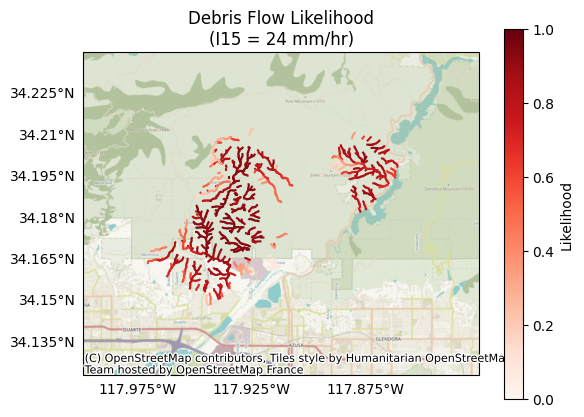
Let’s visualize the results for a design storm with a peak 15-minute rainfall intensity of 6 mm/hour (likelihoods[:,1]):. This is equivalent to a design storm with a peak 15-minute intensity of 24 mm/hour:

k = 1  # The index of the design storm we are plotting
plot.likelihood(segments, likelihoods[:,k], title='Debris Flow Likelihood', I15=I15_mm_hr[k], clabel='Likelihood')

Combined Hazard

Now that we’ve estimated likelihoods and sediment volumes, we can classify each segment’s combined relative hazard. We’ll use a modified version of the classification presented by Cannon et al., 2010. In brief, this model considers a segment’s likelihood and volume results and assigns the segment a score of 1, 2, or 3, which indicate the following:

Value	Relative Hazard
1	Low hazard
2	Moderate hazard
3	High hazard

You can implement this model using the models.c10 module:

from pfdf.models import c10

The original model uses 3 likelihood thresholds, but we’ll use the p_thresholds variable to use 4 thresholds instead:

p_thresholds = [0.2, 0.4, 0.6, 0.8]

We can then classify combined hazards using the hazard function:

hazards = c10.hazard(likelihoods, volumes, p_thresholds=p_thresholds)

The output is a 2D array with one row per segments, and one column per design storm:

print(hazards.shape)
print((segments.size, len(R15)))

(460, 4)
(460, 4)

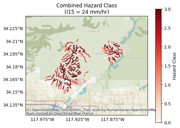
Let’s inspect the results for a design storm with a peak 15-minute rainfall intensity of 24 mm/hour:

k = 1  # The index of the design storm we are plotting
plot.hazard(segments, hazards[:,k], title='Combined Hazard Class', I15=I15_mm_hr[k], clabel='Hazard Class')

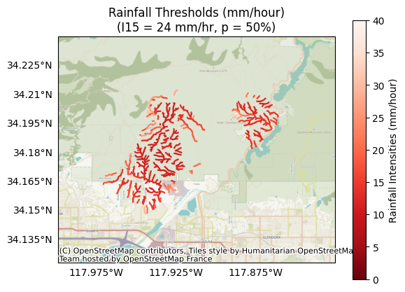
Rainfall Thresholds

Finally, we’ll run a rainfall threshold model - specifically, the inverted M1 likelihood model. Unlike the volume and likelihood models, the rainfall threshold model does not use design storms as an input, so we’re not tied to the design storms used by the volume model. Instead, we’ll run the rainfall threshold model for 15, 30, and 60 minute rainfall durations:

durations = [15, 30, 60]

We’ll also define the design probability levels used to estimate rainfall thresholds. Here, we’ll estimate thresholds for debris-flow events at the 50% and 75% probability levels:

probabilities = [0.5, 0.75]

We already calculated the terrain, fire, and soil variables when we ran the likelihood model, so we’ll use them again here. However, we previously only acquired calibration parameters for 15-minute rainfall durations. To run the threshold model for multiple rainfall durations, we’ll need to query the calibration parameters for the full set of durations:

B, Ct, Cf, Cs = s17.M1.parameters(durations=durations)

Then, we can run the model using the accumulation function:

accumulations = s17.accumulation(probabilities, B, Ct, T, Cf, F, Cs, S)

The output is a 3D numpy array with one row per stream segment, one column per design probability, and one page per rainfall duration:

print(accumulations.shape)
print((segments.size, len(probabilities), len(durations)))

(460, 2, 3)
(460, 2, 3)

The M1 model returns rainfall accumulations when inverted, but many users prefer working with rainfall intensities instead. Before continuing, we’ll use the intensity module to convert the accumulations to intensities:

intensities = intensity.from_accumulation(accumulations, durations=durations)

Inspecting the first element in the two arrays, we find it has been converted from a 15-minute accumulation to a 15-minute intensity. Essentially, the value has been multiplied by 4 to convert mm/15-minutes to mm/hour:

print(accumulations[0,0,0])
print(intensities[0,0,0])

9.323593734639754
37.29437493855902

Let’s inspect the 30-minute thresholds for debris-flow events at the 50% probability level (accumulations[:,0,1]). Here, lower values are more hazardous, as less rainfall is required to trigger debris-flow events:

p = 0  # The index of the probability level
k = 1  # The index of the design storm
plot.thresholds(
    segments, 
    intensities[:,p,k],
    title='Rainfall Thresholds (mm/hour)',
    I15=I15_mm_hr[k], 
    p=probabilities[p],
    clabel='Rainfall Intensities (mm/hour)'
)

Export Results

We’ve illustrated much of this tutorial using matplotlib, but most users will want to export assessment results to a standard GIS file format. For example, as a Shapefile, Geodatabase, or GeoJSON. In this final section, we’ll examine how to export results for:

• Stream segments (LineStrings),

• Basins (Polygons), and

• Outlets (Points)

We’ll do this using the segments.save method, and we’ll include various results from our assessment, including hazard model results, model inputs, and earth-system variables for the segments. We’ll start by creating a folder to hold our exported files:

from pathlib import Path
exports = Path.cwd() / 'exports'
exports.mkdir(exist_ok=True)

Important!

The variables we export in this tutorial are completely arbitrary. You are not required to export these variables in your own code, and you can export many other variables as well. Here, we neglected many variables for the sake of brevity. The field names are also arbitrary - you can use any names you like in your own code.

Tip: File Formats

This tutorial saves results as shapefiles, but you can use most other GIS formats instead. For example, to save results as GeoJSON, change the .shp file extensions to .geojson.

Segments

We’ll start by exporting the stream segments as a collection of LineString features. In addition to the segment geometries, we’d like to include some of our assessment results in the exported shapefile. We can do this by building a properties dict for the export. In general, the keys of the dict should be strings and will be the names of the data fields in the exported file. Each key value should be a 1D numpy array with one element per stream segment.

For the tutorial, let’s export some of the watershed characteristics we used to filter the network, as well as hazard modeling inputs and results. Specifically, let’s export:

Type	Field	Description
Results
	H_24	Hazard score for a design storm of 24 mm/hour
	H_35	Hazard score for a design storm of 35 mm/hour
	H_40	Hazard score for a design storm of 40 mm/hour
	P_35	Debris-flow likelihood for a design storm of 35 mm/hour
	V_35	Potential sediment volume for a design storm of 35 mm/hour
	I_15_50	15-minute rainfall intensity threshold at the 50% probability level
	I_30_75	30-minute rainfall intensity threshold at the 75% probability level
Watershed
	Area	Total catchment area
	BurnRatio	The proportion of catchment area that is burned
Model Inputs
	Terrain_M1	Terrain variable for the M1 model
	Fire_M1	Fire variable for the M1 model
	Soil_M1	Soil variable for the M1 model

Once again, we emphasize that these variables and names are arbitrary. In your own code, you can export any variables you like, and use any field names you like.

Before creating the properties dict, we’ll need to filter our watershed variables. This is because we calculated these variables for the initial stream network, which had many more segments than the final network. Here, we can reuse the keep indices to filter the variables:

area_km2 = area_km2[keep]
burn_ratio = burn_ratio[keep]

We can now build the properties data array. Here, the keys are the names of the data fields in the exported file. Each set of values should be a vector with one element per stream segment, so we will need to index the results arrays to extract relevant results:

properties = {
    # Results
    "H_24": hazards[:,1],
    "H_35": hazards[:,2],
    "H_40": hazards[:,3],
    "P_35": likelihoods[:,1],
    "V_35": volumes[:,1],
    "I_15_50": intensities[:,0,1],
    "I_30_75": intensities[:,1,2],
    # Watershed
    "Area": area_km2,
    "BurnRatio": burn_ratio,
    # Model Inputs
    "Terrain_M1": T,
    "Fire_M1": F,
    "Soil_M1": S,
}

We can now use the save command to save a Shapefile with the segments and their data fields:

path = segments.save(exports/"segments.shp", properties=properties, overwrite=True)
print_path(path)

.../exports/segments.shp

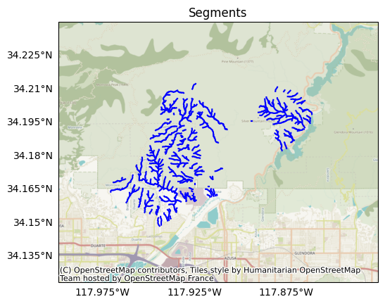
As a reminder, the segments have LineString geometries and resemble the following:

plot.network(segments, title='Segments')

Basins

We’ll next export the outlet basins. The basins have Polygon geometries, and each corresponds to the catchment area for one of the local drainage networks. Most networks will have fewer basins than segments, as there are usually multiple segments in each local drainage network. To export the basins, we’ll use the save command again, but this time we’ll set the type option to basins:

path = segments.save(
    exports/"basins.shp", type="basins", properties=properties, overwrite=True
)
print_path(path)

.../exports/basins.shp

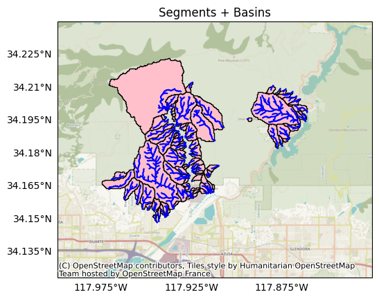
Let’s plot the basins against the segments. Here, stream segments are blue lines, and basins are pink polygons:

from importlib import reload
reload(plot)
plot.network(segments, title='Segments + Basins', show_basins=True)

Outlets

Finally, we’ll export the basin outlets (sometimes referred to as pour points). The outlets have Point geometries, and there is one outlet per basin. Essentially, an outlet is the point in a basin where all flow paths will eventually meet.

Before exporting the outlets, we’ll want to remove any nested drainage basins from the network. A nested basin is an outlet basin that is fully contained within another basin. Nested basins occur when the network breaks flow continuity, and they result in undesirable “hanging” outlet points in the exported dataset. We’ll use the isnested command to identify segments in nested basins, and then remove them with the remove method:

nested = segments.isnested()
segments.remove(nested)

When we export the outlets, we’re not going to include any data properties in the Shapefile. This is usually best practice for outlets, because some outlets can occupy the same spatial point. This occurs, when two basins end at a confluence point - essentially, one outlet is assigned to each of the merging basins, and the two outlets overlap. This can cause confusion when inspecting data fields, as users may unknowingly inspect the wrong outlet for a merging basin. Consequently, we’ll export the outlets without data properties:

path = segments.save(exports/"outlets.shp", type="outlets", overwrite=True)
print_path(path)

.../exports/outlets.shp

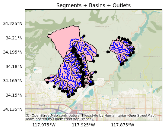
Let’s plot the outlets with the segments and the basins. Here, the outlets are black circles, segments are blue lines, and basins are pink polygons:

plot.network(
    segments, title='Segments + Basins + Outlets', show_basins=True, show_outlets=True
)

Conclusion

In this tutorial, we’ve learned how to use pfdf to implement a hazard assessment. We started by characterizing a watershed - locating burn severity masks, finding flow directions, and computing flow accumulations. We then built a delineation mask and created an initial stream segment network. After characterizing the segments, we refined the network, and we then applied hazards models to each remaining segment. Finally, we exported our assessment results for the segments, basins, and outlets.

This concludes the main tutorial series. At this point, you should have a good grasp of pfdf’s key components, and are probably ready to start writing code. You can find more in-depth discussion of specific components in the advanced tutorials and User Guide, and refer also to the API for a complete reference guide to pfdf.

Quick Reference

This script collects the commands used in the tutorials as a quick reference:

# Resets this notebook for the script
%reset -f

from pfdf.raster import Raster
from pfdf import severity, watershed
from pfdf.segments import Segments
from pfdf.models import g14, s17, c10
from pfdf.utils import intensity

#####
# Parameters
#####

# Network delineation
min_area_km2 = 0.025
min_burned_area_km2 = 0.01
max_length_m = 500

# Network filtering
min_burn_ratio = 0.25
min_slope = 0.12
max_area_km2 = 8
max_developed_area_km2 = 0.025
max_confinement = 174
neighborhood = 4

# Hazard modeling
I15_mm_hr = [16, 24, 35, 40]
durations = [15, 30, 60]
probabilities = [0.5, 0.75]

#####
# Assessment
#####

# Load datasets
perimeter = Raster.from_file('preprocessed/perimeter.tif', isbool=True).values
dem = Raster.from_file('preprocessed/dem.tif')
dnbr = Raster.from_file('preprocessed/dnbr.tif')
kf = Raster.from_file('preprocessed/kf.tif')
barc4 = Raster.from_file('preprocessed/barc4.tif')
iswater = Raster.from_file('preprocessed/iswater.tif', isbool=True).values
isdeveloped = Raster.from_file('preprocessed/isdeveloped.tif', isbool=True)
isretainment = Raster.from_file('preprocessed/retainments.tif', isbool=True)

# Severity masks
isburned = severity.mask(barc4, "burned")
moderate_high = severity.mask(barc4, ["moderate", "high"])

# Watershed characteristics
conditioned = watershed.condition(dem)
flow = watershed.flow(conditioned)
slopes = watershed.slopes(conditioned, flow)
relief = watershed.relief(conditioned, flow)

# Flow accumulations
pixel_area = dem.pixel_area(units='kilometers')
area = watershed.accumulation(flow, times=pixel_area)
burned_area = watershed.accumulation(flow, mask=isburned, times=pixel_area)
nretainments = watershed.accumulation(flow, mask=isretainment)

# Delineation mask
large_enough = area.values >= min_area_km2
below_burn = burned_area.values >= min_burned_area_km2
below_retainment = nretainments.values > 0
at_risk = perimeter | below_burn
mask = large_enough & at_risk & ~iswater & ~below_retainment

# Delineate initial network
segments = Segments(flow, mask, max_length_m)

# Compute segment characteristics
area_km2 = segments.area(units='kilometers')
burn_ratio = segments.burn_ratio(isburned)
slope = segments.slope(slopes)
confinement = segments.confinement(dem, neighborhood)
developed_area_km2 = segments.developed_area(isdeveloped)
in_perimeter = segments.in_perimeter(perimeter)

# Classify segments
floodlike = area_km2 > max_area_km2
burned = burn_ratio >= min_burn_ratio
steep = slope >= min_slope
confined = confinement <= max_confinement
undeveloped = developed_area_km2 <= max_developed_area_km2

# Determine segments that should be retained
at_risk = burned & steep & confined & undeveloped
keep = ~floodlike & (in_perimeter | at_risk)
keep = segments.continuous(keep)

# Filter the netowrk
segments.keep(keep)

# Volume model
Bmh_km2 = segments.burned_area(moderate_high)
relief = segments.relief(relief)
volumes, Vmin, Vmax = g14.emergency(I15_mm_hr, Bmh_km2, relief)

# Likelihood model
B, Ct, Cf, Cs = s17.M1.parameters(durations=15)
R15 = intensity.to_accumulation(I15_mm_hr, durations=15)
T, F, S = s17.M1.variables(segments, moderate_high, slopes, dnbr, kf, omitnan=True)
likelihoods = s17.likelihood(R15, B, Ct, T, Cf, F, Cs, S)

# Combined hazard classification
hazards = c10.hazard(
    likelihoods, volumes, p_thresholds=[0.2, 0.4, 0.6, 0.8]
)

# Rainfall thresholds
B, Ct, Cf, Cs = s17.M1.parameters(durations=durations)
accumulations = s17.accumulation(probabilities, B, Ct, T, Cf, F, Cs, S)
intensities = intensity.from_accumulation(accumulations, durations=durations)

#####
# Export
#####

# Filter watershed variables
area_km2 = area_km2[keep]
burn_ratio = burn_ratio[keep]

# Build property dict
properties = {
    # Results
    "H_24": hazards[:,1],
    "H_35": hazards[:,2],
    "H_40": hazards[:,3],
    "P_35": likelihoods[:,1],
    "V_35": volumes[:,1],
    "I_15_50": intensities[:,0,1],
    "I_30_75": intensities[:,1,2],
    # Watershed
    "Area": area_km2,
    "BurnRatio": burn_ratio,
    # Model Inputs
    "Terrain_M1": T,
    "Fire_M1": F,
    "Soil_M1": S,
}

# Export segments
path = segments.save("exports/segments.shp", properties=properties, overwrite=True)

# Export basins
path = segments.save(
    "exports/basins.shp", type="basins", properties=properties, overwrite=True
)

# Export outlets
nested = segments.isnested()
segments.remove(nested)
path = segments.save("exports/outlets.shp", type="outlets", overwrite=True)